MIT 18.404 — Lecture 6

TM Variants, Church-Turing Thesis

Grades for PSET 1 have been released on Gradescope. We have a quiz next Tuesday (October 6th) from 7:30 PM to 9:00 PM in Walker; sample questions will be posted on the course website.

§ Turing Machines (Recap) & The Church-Turing Thesis

Recall the definition of a Turing machine from Lecture 5. Importantly, for any word $w$ , a Turing machine $M$ can either:

ACCEPT (enter $q_{\mathrm{acc}}$ ) $\parallel$ REJECT BY HALTING (enter $q_{\mathrm{rej}}$ ) $\parallel$ REJECT BY LOOPING (never halt)

The Turing machine will be our model for a general-purpose computer.

Question. Why is a one-tape TM our choice of model? Why not anything else?
(Recall that a PDA with two stacks is strictly more powerful than a PDA with just one stack.)

Answer: As we'll eventually show in this course, it turns out that a one-tape TM is equally as powerful as, say, Python or Java, because one can compile code in any one of these “languages” into any other. In fact…

Theorem. (The Church-Turing Thesis) Any function computable by an “algorithm” is computable by a Turing machine.

(The Church-Turing thesis is more of a heuristic than a theorem.)

Definition. Also recall from Lecture 5 the following properties of languages and TMs.

A Turing machine $M$ is a decider if it halts on every input.
A language $A$ is Turing-recognizable if $A = L(M)$ for some Turing machine $M$ .
A language $A$ is decidable if $A = L(M)$ for some decider $M$ .

§ Multi-Tape Turing Machines

Definition. We say that a multitape Turing machine $M$ is a TM with multiple tapes, naturally.

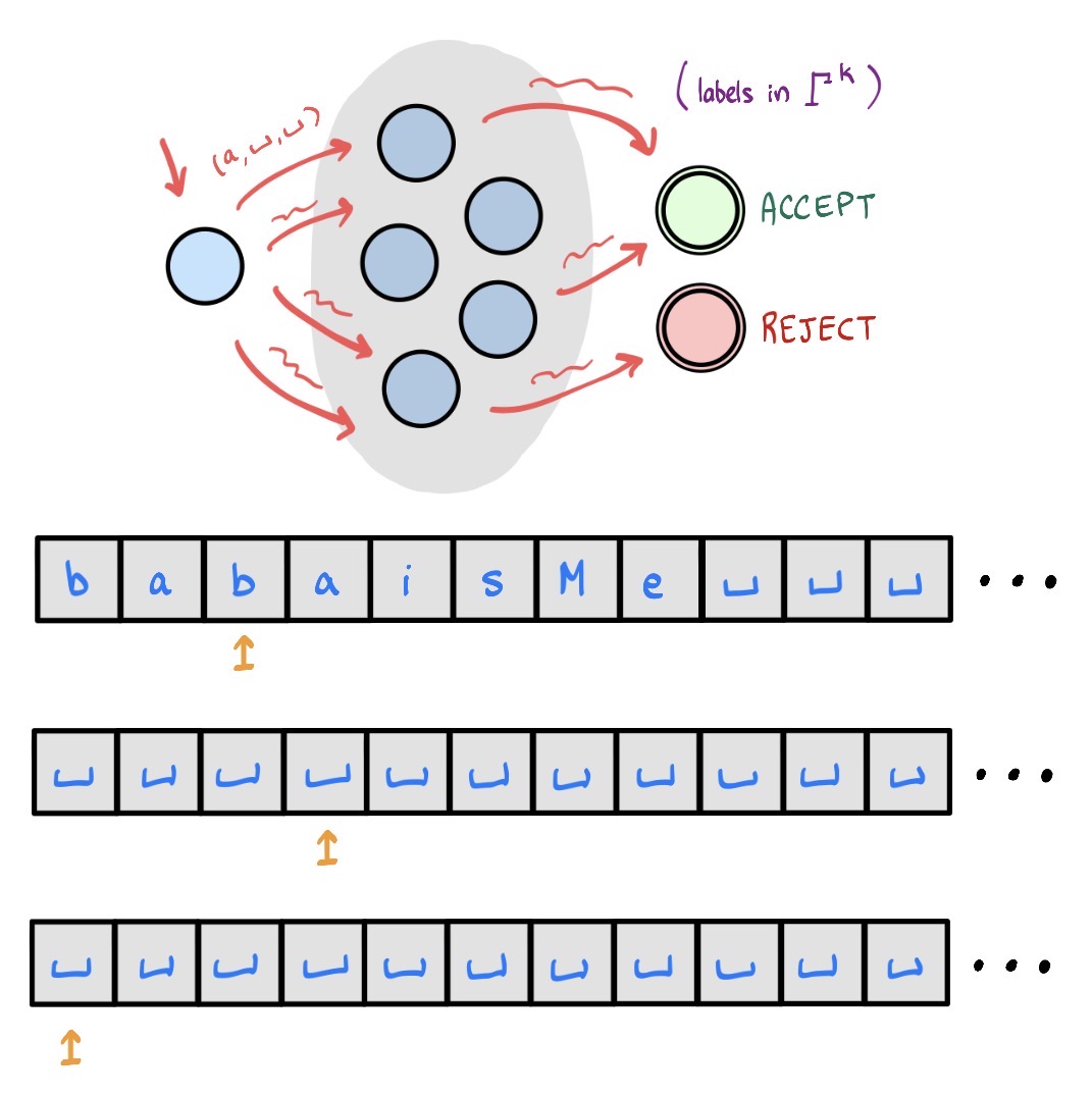
In particular, the transition function of a multitape Turing machine with $k$ tapes has type $\delta \colon Q \times \Gamma^k \to Q \times \Gamma^k \times \{\mathrm{L}, \mathrm{R}\}^k$ .

Theorem. (Multitape = Single Tape) A language $A$ is Turing-recognizable if and only if $A = L(M)$ for some multitape TM $M$ .

Proof: The $\implies$ direction is obvious. For the $\impliedby$ direction, a one-tape TM $S$ can simulate a multitape TM $M$ like so.

The idea is to simply store the concatenation of all $k$ tapes in a single tape.

Separate each of the $k$ tapes with a $\str{\#}$ symbol.
- If one of the $k$ tapes writes in a blank space—thereby “extending its length”—then we simply shift everything to the right.
Keep track of the head position on each of the $k$ tapes by writing $\str{c}^{\bullet}$ if the head is pointing to $\str{c}$ .

Details omitted, but they're not hard to implement. $\blacksquare$

Remark. It follows that “a PDA with 100 stacks plus a tape” is equally as powerful as “an FA plus a tape”.

§ Nondeterministic Turing Machines

Definition. We say that a nondeterministic Turing machine (NTM) $M$ is a TM that's nondeterministic, naturally. The transition function has type $\delta \colon Q \times \Gamma \to \mathcal{P}(Q \times \Gamma \times \{\mathrm{L}, \mathrm{R}\})$ .

Theorem. (NTM = TM) A language $A$ is Turing-recognizable if and only if $A = L(N)$ for some NTM $N$ .

Proof: The $\implies$ direction is obvious.

For the $\impliedby$ direction, the idea is for a one-tape TM $M$ to BFS through the tree of computation paths of $N$ .

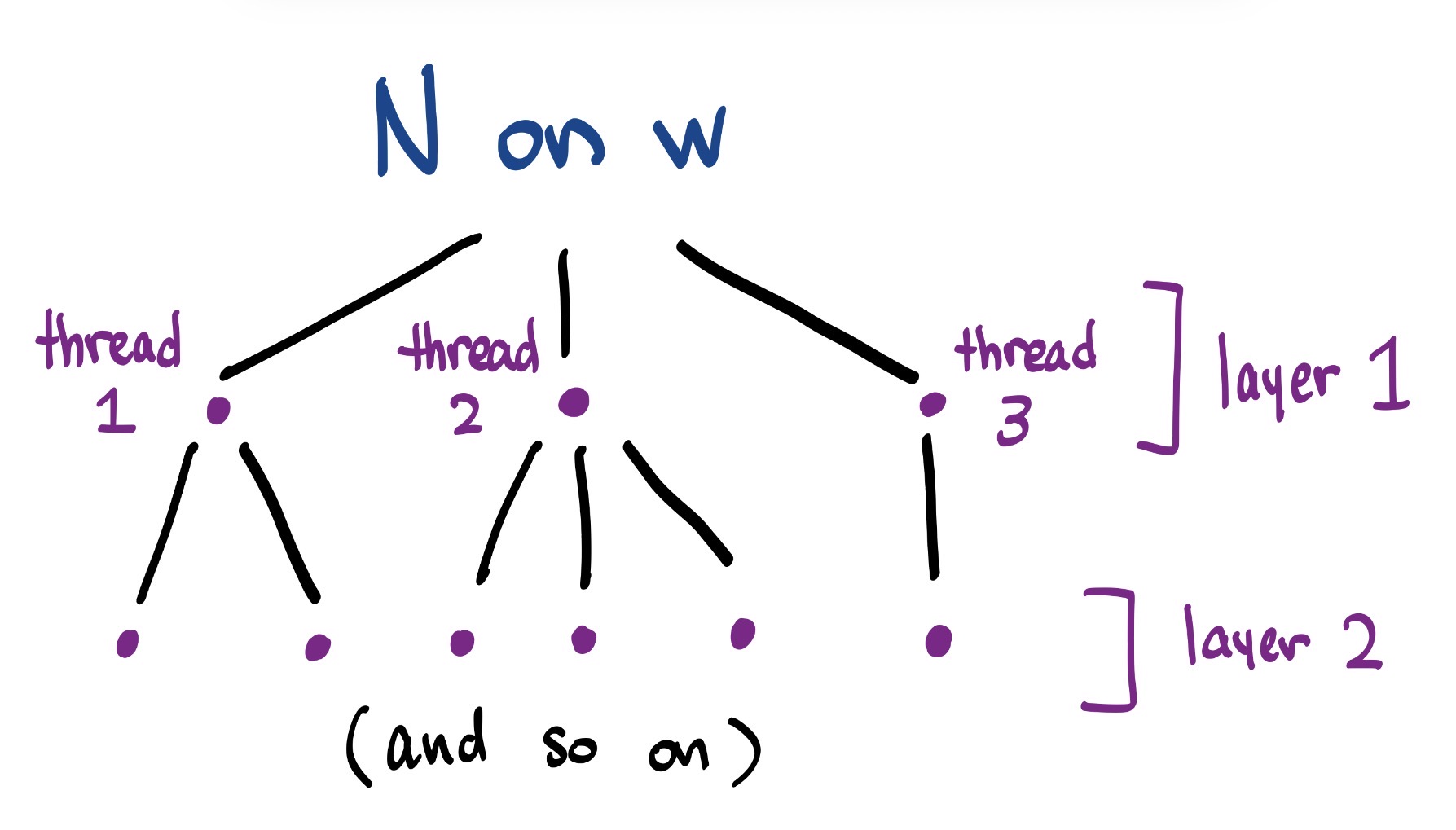
In the single tape of $M$ , we simply store the state of all threads of $N$ , moving down one layer at a time.

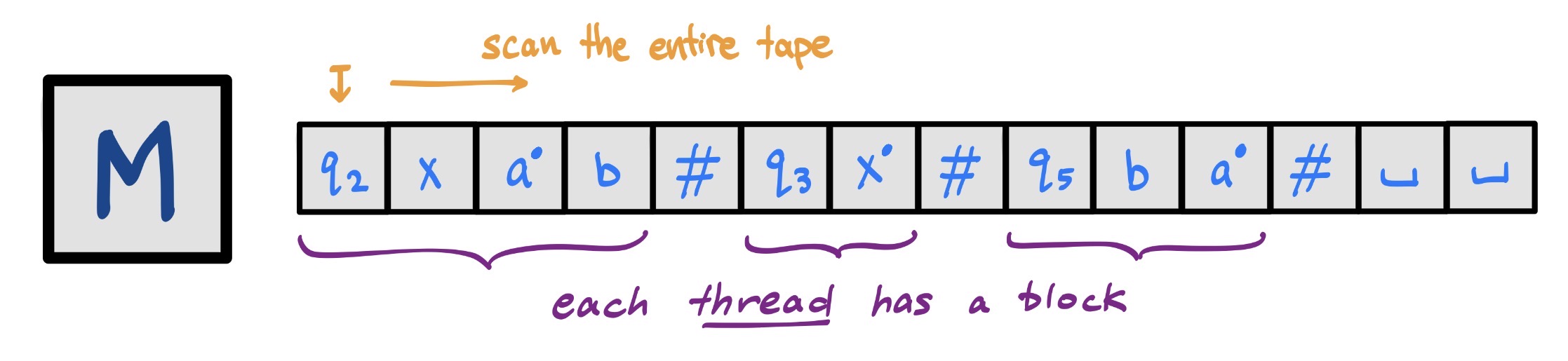
As before, threads are separated with $\str{\#}$ , and tape heads are indicated by the $\bullet$ in $\str{c}^{\bullet}$ . Furthermore, each block begins with a cell that stores the FA state that the thread lands at (e.g., $q_2$ , $q_3$ , or $q_5$ , as shown above).

So the TM should BFS through all threads layer-by-layer and return $\str{ACCEPT}$ if any thread returns $\str{ACCEPT}$ . (Details omitted.) $\blacksquare$

§ Enumerators (Turing Machines with Printers)

Definition. We say that an enumerator $E$ is a Turing machine that takes no inputs and prints outputs. Specifically,

Its workspace tape is initially completely empty.
At any point, $E$ can move to a $\str{print}$ state and print the contents of the workspace.

We let $L(E)$ denote the set of strings that $E$ eventually prints.

Theorem. (Enumerator = TM) A language $A$ is Turing-recognizable if and only if $A = L(E)$ for some enumerator $E$ .

Proof: We first consider the $\impliedby$ direction: given any $A$ for which $A = L(E)$ , we construct a TM $M$ for which $A = L(M)$ .

Solution: On input $w$ , simply simulate $E$ on a blank tape. During the simulation, check everything it prints for whether it matches $w$ . If there's ever a match, return $\str{ACCEPT}$ . $\square$

Now for the $\implies$ direction: given any $M$ for which $A = L(M)$ , we construct an enumerator $E$ that prints out $A$ .

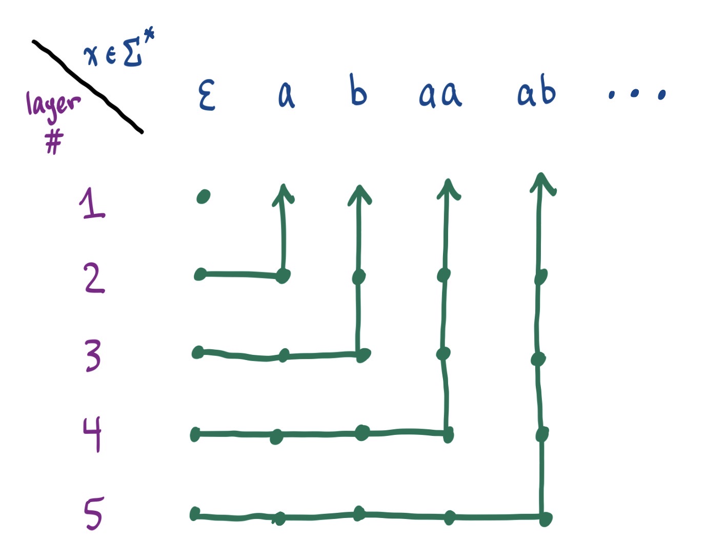
Solution: The rough idea is brute force: for each $x \in \Sigma^*$ , simulate $M$ on $x$ , and print $x$ if $M$ accepts. There are two issues:

If we try to simulate one $x \in \Sigma^*$ at a time, then we might fail if a simulation of $M$ on $x$ loops.
If we try to simulate one layer at a time, then we'll never get past the first layer because $\Sigma^*$ is infinite.

(In a rough sense, the former is DFS, and the latter is BFS—but this time, they both fail.)

The fix is similar to how we prove $|\mathbb{Q}| = |\mathbb{N}|$ ; do a “zig-zag” across both $\Sigma^*$ and layers, like so.

More formally, in the $i^{\text{th}}$ step, run $(x_1, x_2, \dots, x_i)$ up to the $i^{\text{th}}$ layer, and do this for all $i \in \mathbb{N}$ . $\square$

This completes the proof of both directions. (Again, many details omitted.) $\blacksquare$