MIT 6.1220 — Lecture 10

Maximum Flow (Part II)

Let's first analyze the runtime of our Ford-Fulkerson algorithm.

Solution. (Ford-Fulkerson) Repeatedly find augmenting paths $P := s \to \dots \to t$ , then recompute the residual network each time. Repeat until no more augmenting paths exist. This is optimal.

Suppose all capacities are integers in $[0, C]$ , so our algorithm actually terminates.

Computing $G_f$ at each step takes $O(|E|)$ .
Searching for an augmenting path at each step takes $O(|E|)$ .
The number of steps is at most the max flow $F^*$ . This is:
- Lower-bounded by the number of augmentations, and…
- Upper-bounded by the cut of the cut $\{s\}$ , which is upper-bounded by $|V| \cdot C$ .

So overall, we have a runtime of $O(|E| \cdot |V| \cdot C)$ , or $O(|E| \cdot F^*)$ where $F^*$ is the max flow.

Remark. This is a pseudopolynomial runtime; we can still get pseudopolynomial runtime with rational capacities! But real-numbered capacities might yield an infinite loop, so this is the best we can do.

However, if we choose our paths poorly, Ford-Fulkerson can have needlessly long runtime.

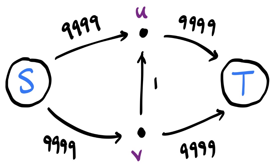
If Ford-Fulkerson picks paths $s \to u \to t$ and $s \to v \to t$ , it can finish in just two steps.
But it might also finish in $19998$ steps if it picks paths $s \to v \to u \to t$ and $s \to u \to v \to t$ .

Solution. (Better Ford-Fulkerson) Repeatedly find the highest bottleneck capacity augmenting path $s \to t$ , and recompute the residual network each time.

How? Dijkstra's, but store the minimum encountered edge weight at each vertex. This takes $O(|E| \log |V|)$ time.

To analyze the runtime of this algorithm, we make the following claim.

Claim. For any graph $G$ with max flow $F^*$ , there exists a path $s \to t$ with bottleneck capacity at least $\frac{F^*}{|E|}$ .

Proof: Flow Decomposition Lemma. When decomposing a flow into paths and cycles, every path / cycle created will “use up” at least one of the $|E|$ edges. So the flow can be decomposed into at most $|E|$ paths and cycles.

Now apply a probabilistic argument. $\blacksquare$

Now for the runtime of Better Ford-Fulkerson.

Claim. The better Ford-Fulkerson runs in $O(|E|^2 \cdot \log |V| \cdot \log (C \cdot |V|))$ time.

Proof: Each step takes $O(|E| \cdot \log|V|)$ time (finding the maximum bottleneck path). Also, each step cuts the remaining flow down by a factor of $1 - \frac{1}{|E|}$ , so the total number of steps is upper-bounded by $O(|E| \cdot \log(C \cdot |V|))$ . The end. $\blacksquare$

The gain here is that the dependence on $C$ is now logarithmic, not linear. This is weakly polynomial runtime.

It turns out we have other solutions.

Solution. (Edmonds-Karp) Repeatedly find the shortest (least # of edges) augmenting path $s \to t$ , and recompute the residual network each time. How? BFS.

This has runtime $O(|E|^2 \cdot |V|)$ , with no dependence on $C$ .

Solution. (Chen Kyng Liu … '22) You can solve this problem in $O(|E|^{1 + o(1)} \cdot \log C)$ time.

We'll end with an application of our newfound max-flow-finding tech.

Problem. (Bipartite Matching) Given a bipartite graph $L \sqcup R$ , find the largest possible matching.

Solution. (Bipartite Matching) Construct $s$ and $t$ , then direct all edges $s \to L \to R \to t$ and give them weight $1$ . Then the maximum flow yields the largest possible matching. (How is the “matching” constraint enforced?) $\blacksquare$