MIT 6.7960 — Lecture 5
Architectures: Sequence Modeling
§ Sequence Modeling
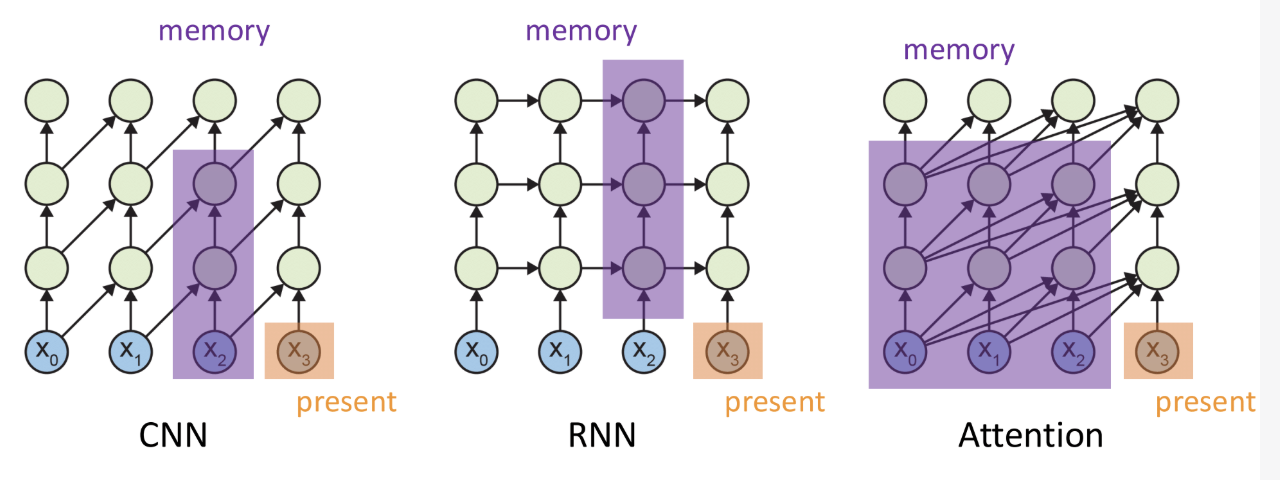
We spend the first 10 minutes stating that sequence modeling involves a model that retains memory, thereby deciding its output and updating its memory at each time step as a function of its memory and its present input.
In this lecture, we'll discuss the CNN and RNN paradigms; we'll talk about attention and transformers next time.
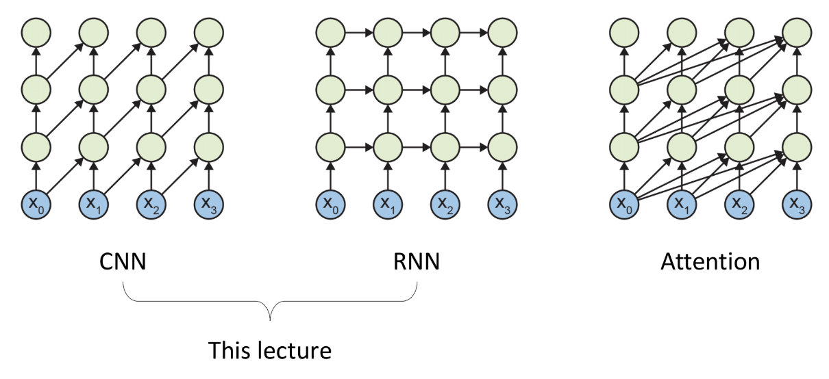
§ Causal CNNs
The architecture of causal CNNs looks exactly as you'd expect.
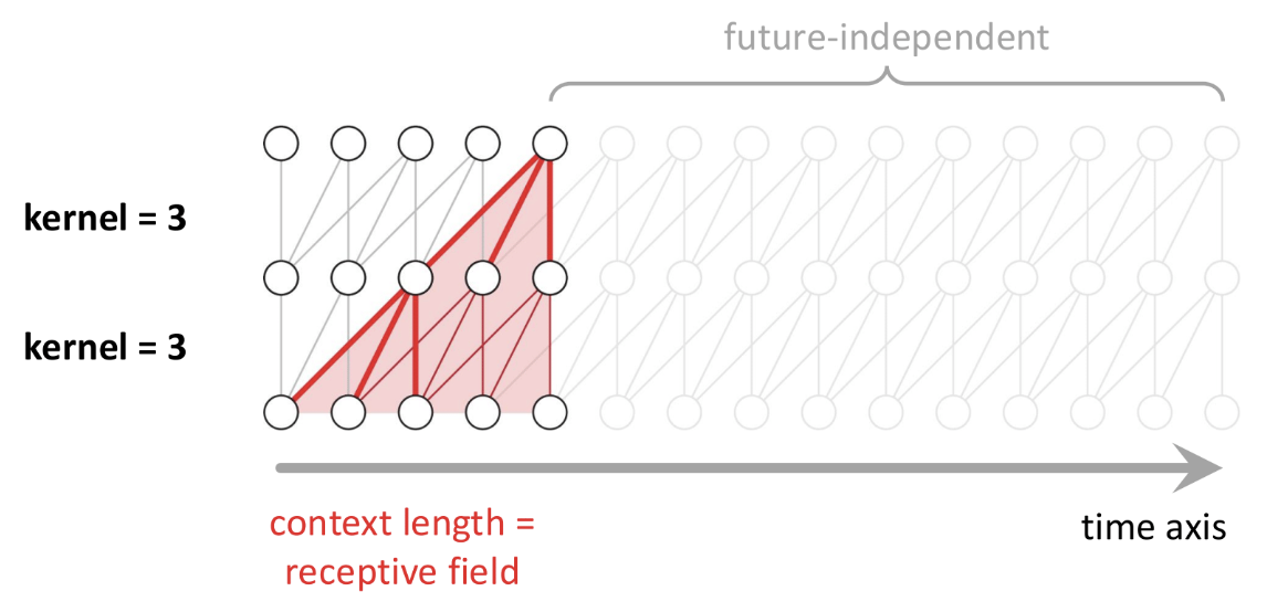
Rather than taking hidden layers to be convolutions across space, we take hidden layers to be convolutions across time. In some sense, the architecture has no fixed size of its input layer; the size of its input layer grows as time grows.
Remark. Though in another sense, the size of the relevant input layer is bounded by the context length.
Note that there is weight-sharing: the kernel used to get from the input layer to the first layer remains invariant as time passes.
§ Recurrent Neural Networks (RNNs)
Wow, we've already burnt half an hour! Here's how the architecture of causal RNNs works.
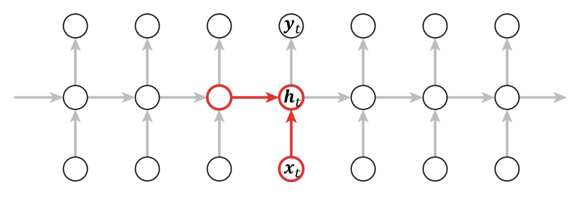
The idea is that depends not just on the input , but also on a state that updates every time step.
Thus, to specify an RNN, one must specify and . Pictured below is a possible choice of and .
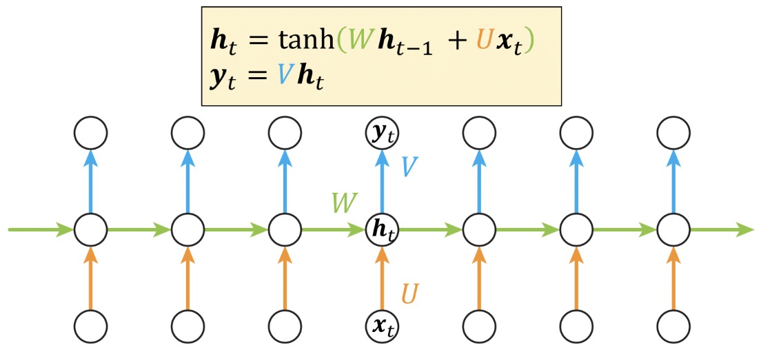
One reason for using to compute state is that it is zero-centered.
Remark. I feel like a 10-year-old could understand the level of depth taught in this class.
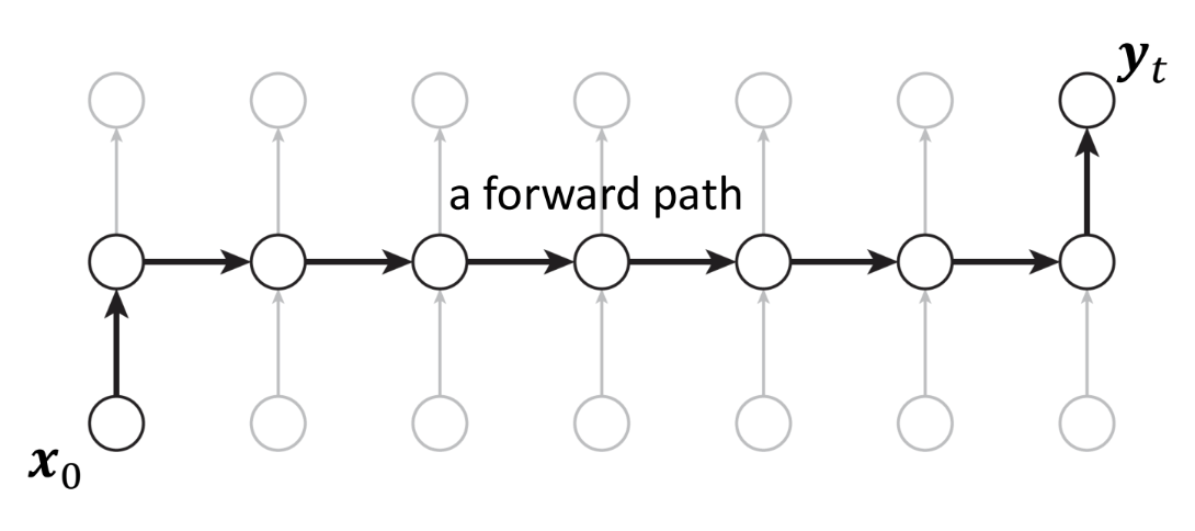
Here's what forward passes look like in RNNs.
And wow! Here's what the backward pass looks like!
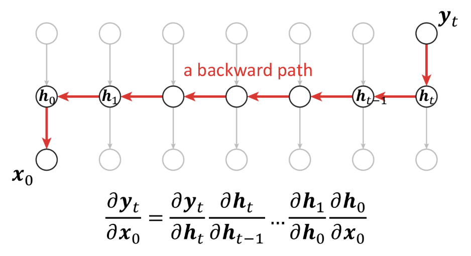
What a surprise! It's now been almost an hour, and we've already covered 5 pages of a picture book!
§ Long Short-Term Memory (LSTM)
There's a problem with our RNN design.
In practice, we cannot take backward passes over such long distances, because we will have either exploding or vanishing gradients, since we are taking products of arbitrarily-large numbers of terms.
One partial fix is to use the Long Short-Term Memory (LSTM) architecture. First, we must spend a full minute reviewing the meanings of the words “long”, “short-term”, and “memory”, for those who joined late and don't understand slang.
Here's the architecture of an LSTM.
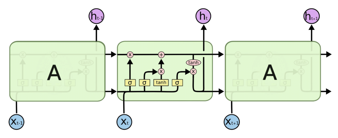
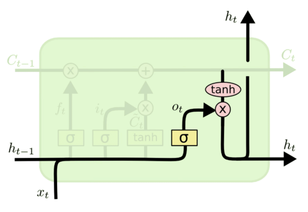
Each cell of the LSTM takes in an input , the previous cell's hidden state , and the previous cell's cell state .
We now discuss the architecture of each cell; throughout this discussion, it helps to recall that is like a 0/1 switch, whereas maps values into .
The cell state is .
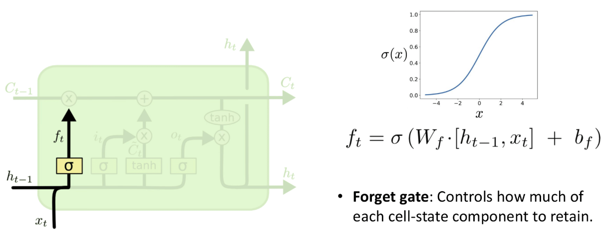
The forget weight is given by .
The learn-information weight is given by .
The new information being learned is given by .
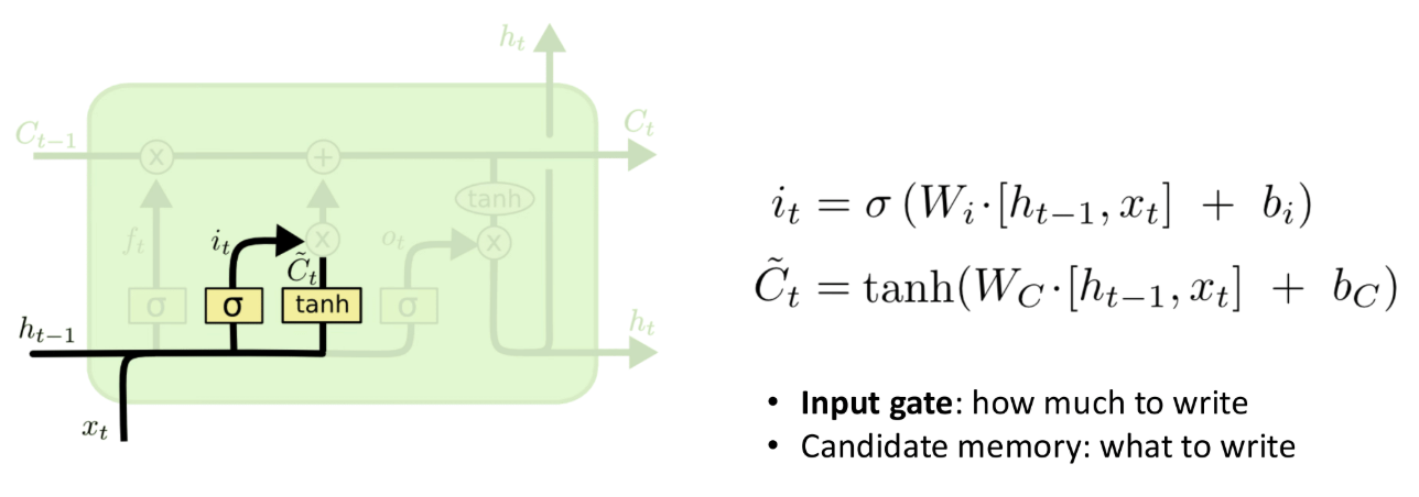
The hidden state is , where .
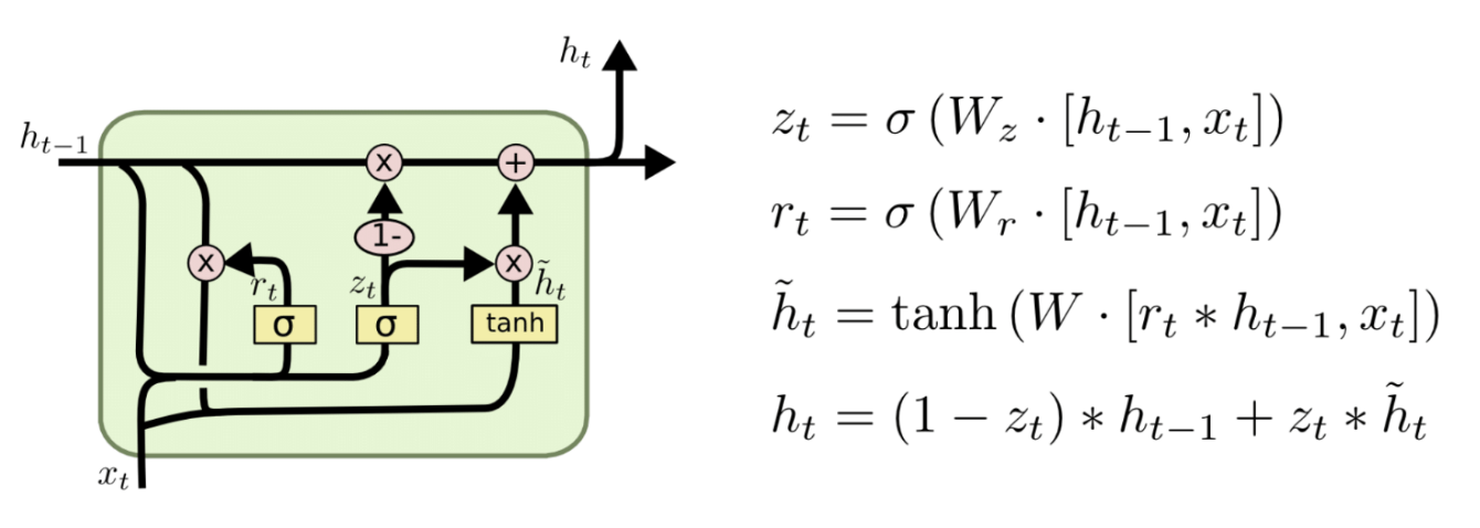
There are variations of the LSTM architecture, too, such as the GRU below, which has a hidden state but no cell state.
Historically, the LSTM and GRU were go-to architectures for RNN models because they mitigated vanishing-gradient problems. Nowadays, though, transformers are the favored architecture.
§ Deep RNNs
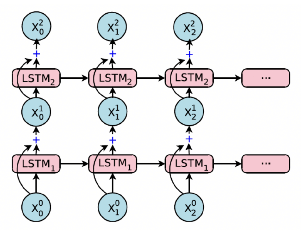
You can also make deep RNNs. They look and work how you'd expect.
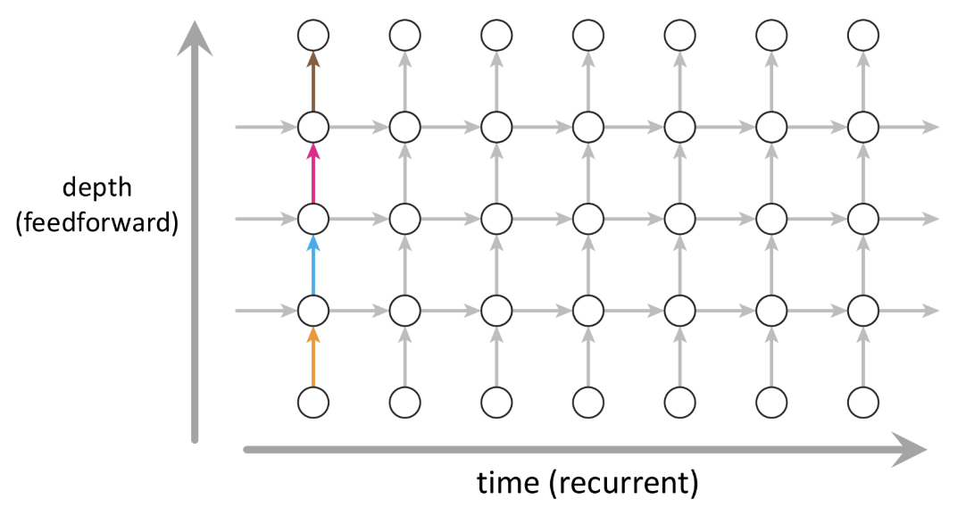
And you might integrate the LSTM stuff with this, too, as used by Google in 2016.
Wow. Amazing.
§ Advantages and Disadvantages
This slide says it all.
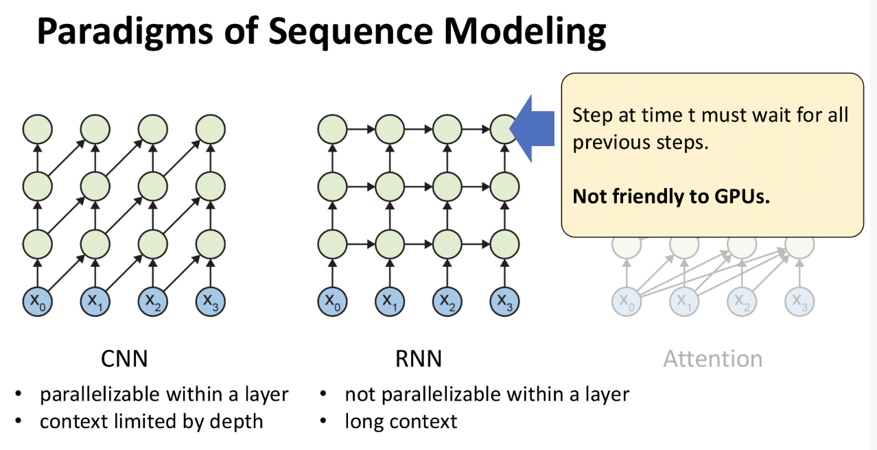
The lecture just reads off this slide.
§ Memory
This slide says it all.
I'm leaving now.