MIT 6.7960 — Lecture 2

How to Train a Neural Net

§ Gradient-Based Optimization

Gradient descent isn't the only gradient-based optimization algorithm. Even if we can compute the gradient $\mathbf{g} = \nabla_{\theta} J(\theta)$ of a neural net, what should we do with it to best minimize the objective?

\theta^{k + 1} \gets \theta^k + \eta \cdot \textsc{Update}(\mathbf{g})

In general, any optimization algorithm must effectively define the following two things.

A surrogate—a local approximation of the loss function.
- Example. We might take a first-degree Taylor approximation of the loss.
A trust region—a region in which the surrogate is trustable.
- Example. We might take the trust region to be a $\lambda$ -radius ball.

If we use the two examples given above, we get exactly gradient descent:

\argmin_{\|\Delta \mathbf{w}\|_2 \le \lambda} \mathbf{g}^{\top}\Delta \mathbf{w} = -\lambda \cdot \frac{\mathbf{g}}{\|\mathbf{g}\|_2}.

But we can also generalize—if we take the trust region to be a $\lambda$ -radius square, we get a different optimizer.

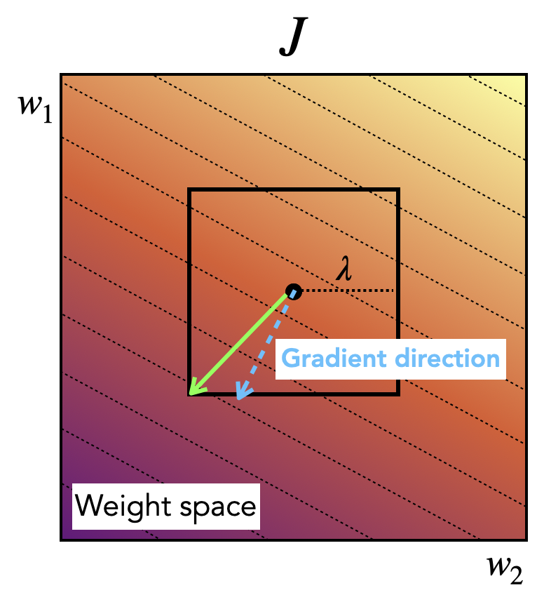
This optimizer is called sign descent because the minimizer looks like this:

\argmin_{\|\Delta \mathbf{w}\|_{\infty} \le \lambda} \mathbf{g}^{\top}\Delta \mathbf{w} = -\lambda \cdot \mathrm{sign}(\mathbf{g}).

We can also set the trust region using the spectral norm of the weight update, which produces spectral descent.

\argmin_{\|\Delta W\|_{\mathrm{op}} \le \lambda} \langle G, \Delta W \rangle = -\lambda \cdot UV^{\top} ~~~ \text{ where } ~~~ G = U\Sigma V^{\top}.

Remark. Lecture did not give any elaboration on what spectral descent is. In short, the spectral norm of a matrix is its largest singular value (see Lecture 19 of 18.701), so $-\lambda \cdot UV^{\top}$ is just $-G$ with every singular value flattened to $\lambda$ .

§ Bells and Whistles

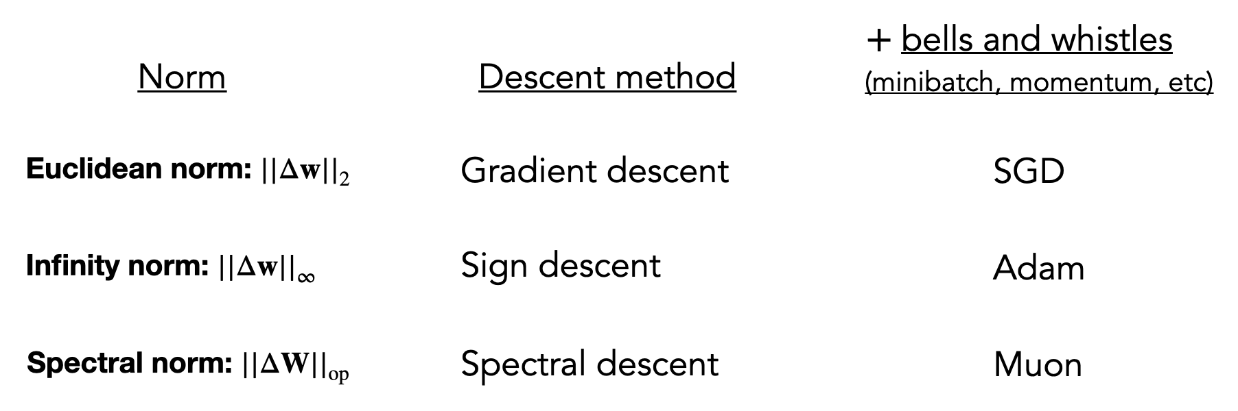
It turns out that sign descent and spectral descent (with bells and whistles) both yield commonly-used descent methods.

Stochasticity. The gradient is computed by averaging across only a subset of the data.

Advantages: It's much cheaper, and the noise of the stochasticity serves as an implicit regularizer.
Disadvantages: Higher variance due to gradient approximation.

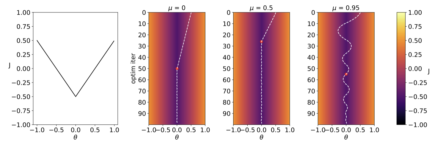
Momentum. Say the gradient steps are biased to continue in the direction of the previous update.

\theta^{t + 1} \gets \theta^t - \eta \nabla f(\theta^{t}) + \alpha \cdot m^t ~~~ \text{ where } ~~~ m^t = \theta^t - \theta^{t - 1} \text{ is the previous update.}

Expectedly, the constant $\alpha$ needs to be tuned carefully, or else advantages may become disadvantages.

§ Gradient Difficulties

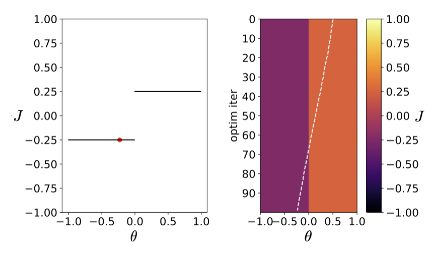
Some functions are easier to optimize than others.

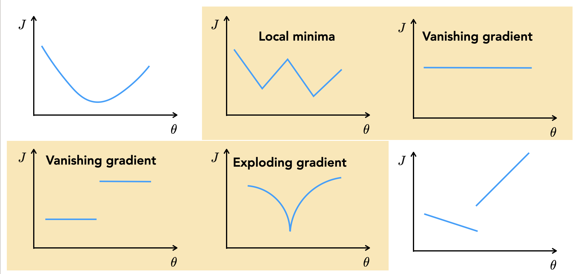
Note that even though most of these functions are not differentiable, they all have gradients in PyTorch. Even then, though, PyTorch cannot find a global minimum when there are vanishing gradients, exploding gradients, or local minima.

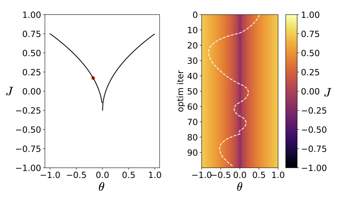
One fix is to use gradient clipping: if gradients exceed a magnitude $M$ , scale them to have magnitude $M$ .

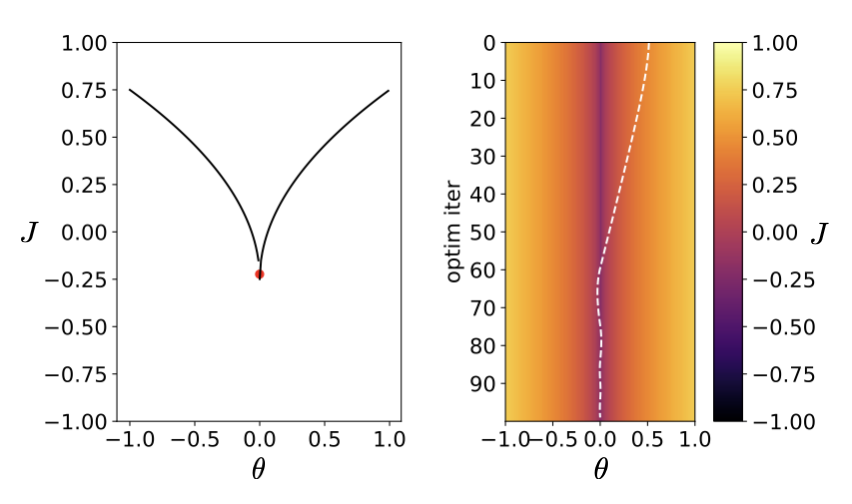
Another fix is to choose a direction not by computing the gradient, but by considering small perturbations of $\theta$ in all directions and moving in the direction of lower loss.

§ Backpropagation

See Lecture 13 of 6.790 for an explanation of backpropagation specifically when each layer's computation $f(\mathbf{x}_{\mathrm{in}}, \theta)$ is a linear layer plus an activation. We give a more general description here. (Below, $\theta$ and $\mathbf{W}$ are synonymous.)

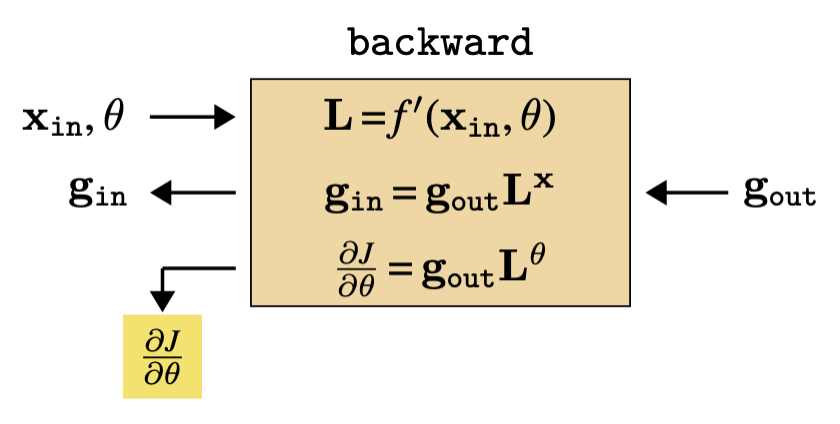
Notably, for linear layers we have $f(\mathbf{x}_{\mathrm{in}}, \mathbf{W}) = \mathbf{W}\mathbf{x}_{\mathrm{in}}$ , so it follows that $\mathbf{L}^{\mathbf{x}} = \mathbf{W}$ and $\mathbf{L}^{\theta} = \mathbf{x}_{\mathrm{in}}$ . So backprop is easy.

In practice, not all layers are linear, of course. For example,

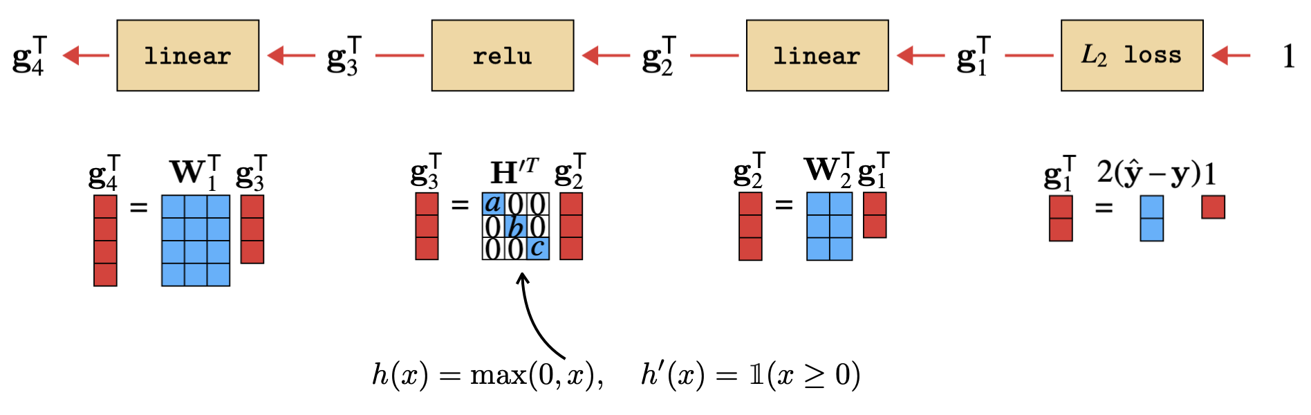
But the nonlinear layers like relu are also easy to deal with—relu's Jacobian $\mathbf{L}^{\mathbf{x}}$ is diagonal.

And of course, all of this is compatible with more general features of DAGs, like merges and branches.

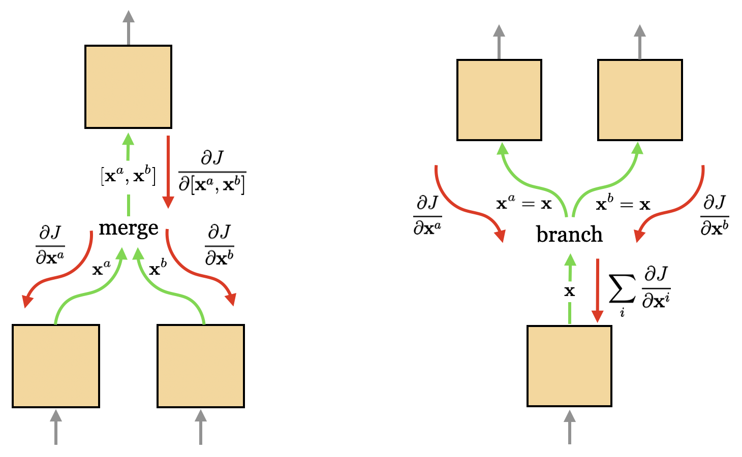
Note that parameter sharing (used in CNNs, e.g.) is just a variant of branching.