MIT 6.7960 — Lecture 9

§ Representations

Solving hard problems oftentimes requires finding good representations.

• The game of Go was thought to be very hard because it has $3^{19 \times 19}$ possible states.

• Image analysis was thought to be very hard because it has $256^{3 \times 500 \times 500}$ possible states (say).

But we've seen in Lecture 4 that there are tricks that improve our representation of an image—specifically, our representation consists of convolutions of the image.

Definition. Given a data domain $\mathcal{X}$, a representation is a function $f \colon \mathcal{X} \to \mathbb{R}^d$ that assigns a feature vector to each input $x \in \mathcal{X}$.

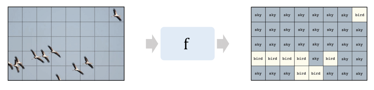
Example. We might represent an image with one-hot vectors, where each vector states which cells contain, say, a bird.

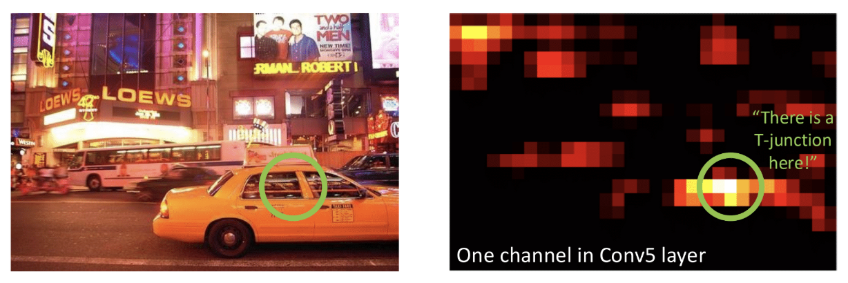
Alternatively, one part of a representation might answer whether each cell of an image contains, say, a T-junction.

And, of course, we can chain representations together.

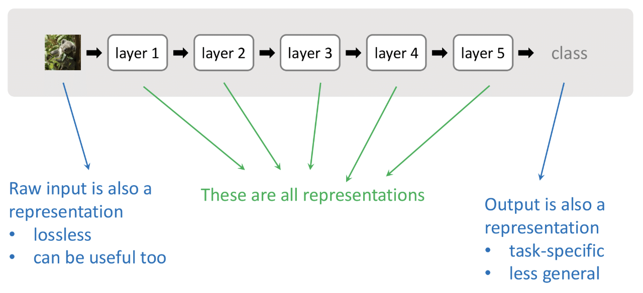
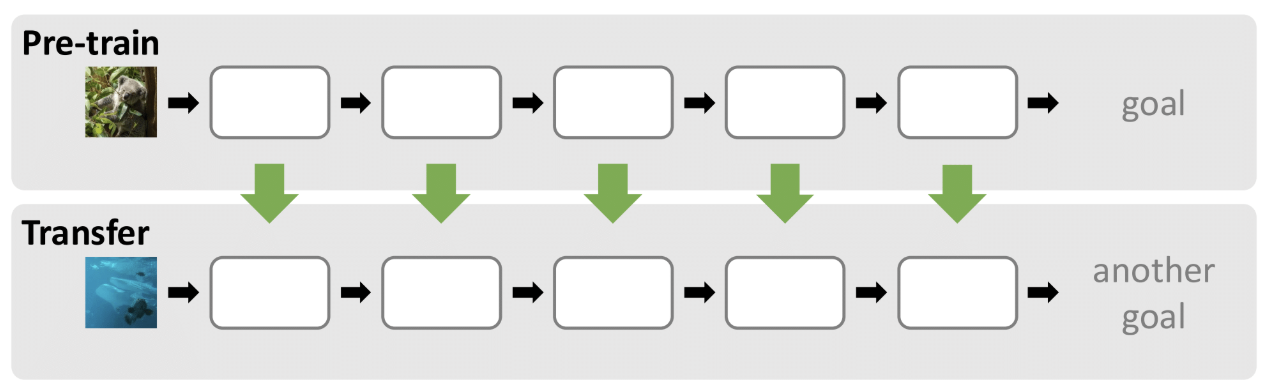
In fact, we can also transfer representations; not only can a model learn things about its data set, but it can also learn representations that might be useful for other data sets, too!

§ Unsupervised Learning: Auxiliary Targets

Traditional learning methods (i.e., supervised learning) require data $X$ that is labeled with outputs $Y$.

But labeling data costs time and money, and the results can be biased. What if we could still learn things without labels—some sort of unsupervised learning, perhaps?

Well, as we just saw in the previous section, representations are learnable even on unlabeled data sets, particularly if the auxiliary target used for the unlabeled data sets does not require labels.

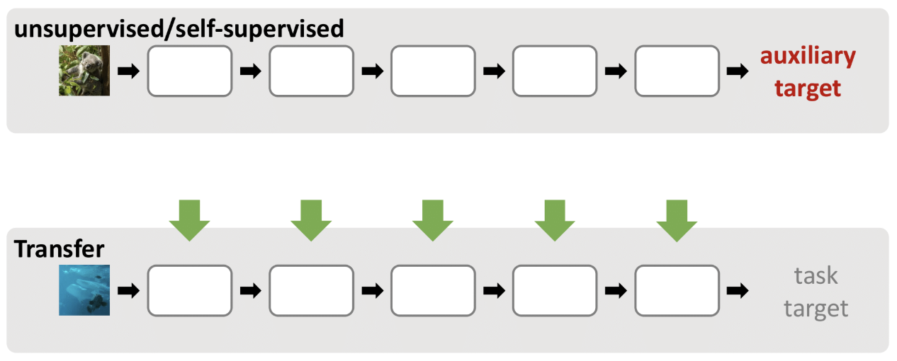
There are two main kinds of auxiliary targets (i.e., ways to define a loss for our representation).

• Reconstruction-based. How much does the data change when it is encoded and then decoded?

  

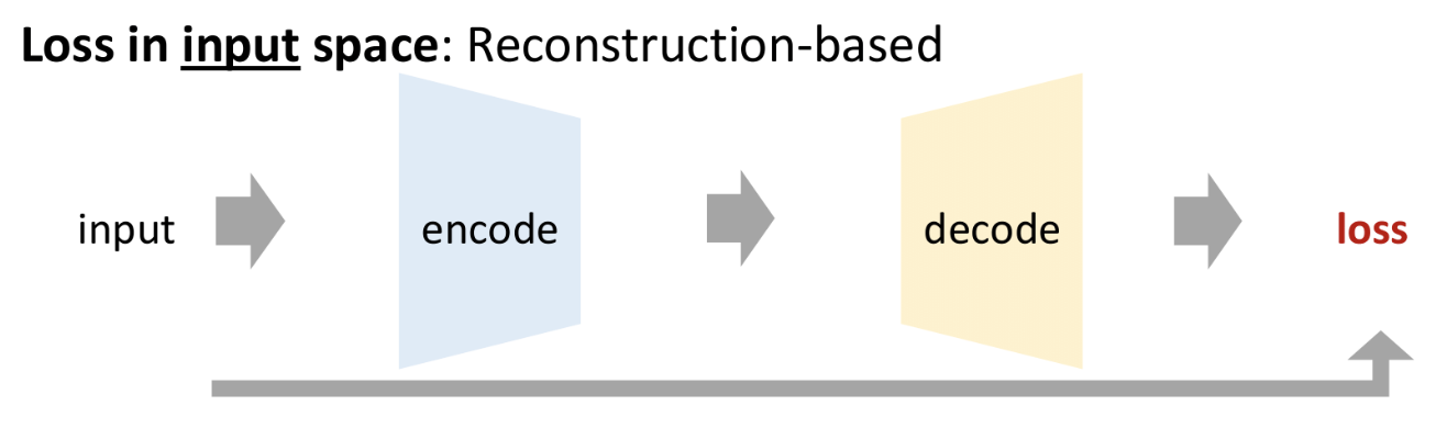
  Here, loss is defined in the input space.

• Similarity-based. Is the difference between two inputs similar to the difference between their encodings?

  

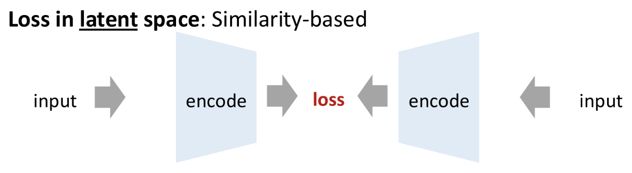
  Interestingly, loss is defined here in the latent space.

§ Reconstruction-Based Methods

We discuss three learning methods that work well with reconstruction-based learning.

K-means Clustering. Given some data, we want to group it into $k$ clusters based on proximity.

1. Our representation will be a set of $k$ $\underline{\text{centers}}$ $\{c(i)\}_{i = 1}^k$, so that $x$ is in the $i^{\text{th}}$ cluster if the center closest to it is $c(i)$.

2. First, initialize $\{c(i)\}_{i = 1}^k$ randomly.

3. Then repeatedly replace each center $c(i)$ with the centroid of its cluster.

The loss of a clustering is given by:

$$\mathcal{L}(\{c(i)\}) := \sum_{x \in X} \|x - c(i(x))\|^2 = \sum_{x \in X} \|x - D(E(x))\|^2 \text{ where } D \text{ is the decoder and } E \text{ is the encoder.}$$

Notice how, as indicated by the expression above, the loss of k-means clustering matches that of reconstruction-based loss.

Blobs Uneven Rings

Random k-means++

Step Run Reset

Loss L = 1N ∑_x ‖x − c(x)‖² (mean squared distance to the assigned center) after assignment after update

k

4

You can see k-means clustering in action using the (warning: AI-generated) widget above.

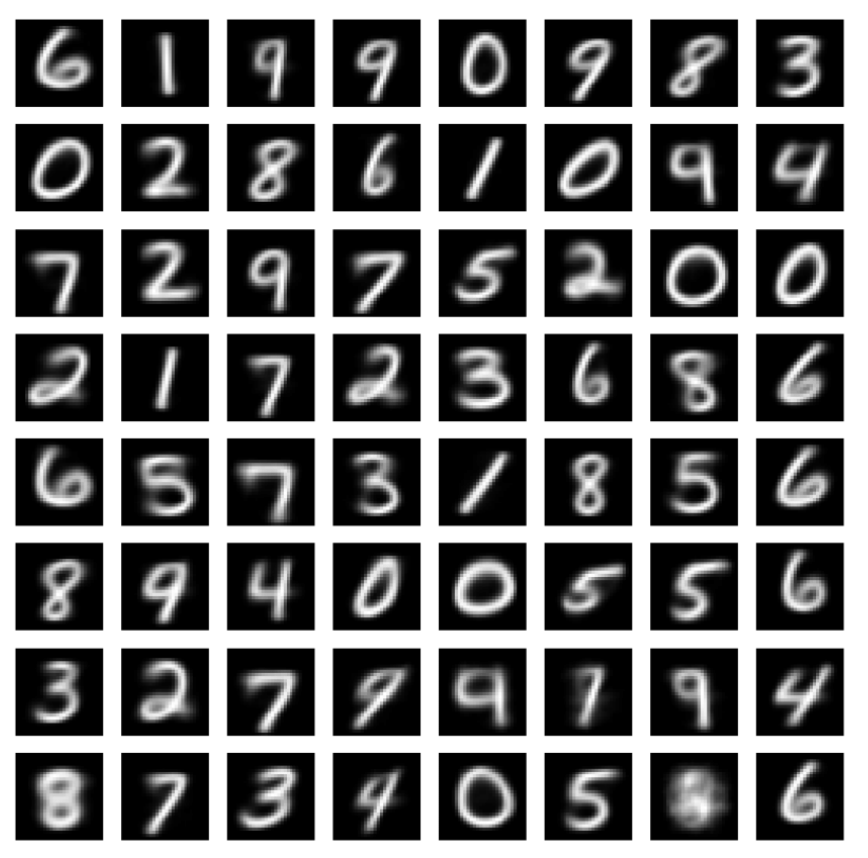
A k-means clustering representation for MNIST digits is a collection of $k$ centers, where each center is an image. Here's how the result might look for $k = 64$, for example.

Principal Component Analysis (PCA). Recall Lecture 19 of 18.701. The point is that:

• Say $W_k \in \mathbb{R}^{d \times k}$ is a matrix consisting of the $k$ eigenvectors of $X^{\top}X$ with largest eigenvalue.

• Our encoder then takes $x$ and expresses it in the coordinates of the principal basis: $x \mapsto W_k^{\top}x$.

• Our decoder just undoes this map: $z \mapsto W_k z$.

The loss of PCA is given by:

$$\mathcal{L}(W_k) := \|X - XW_kW_k^{\top}\|_F^2 = \sum_{x \in X} \|x - D(E(x))\|^2, \text{ where } D \text{ is the decoder and } E \text{ is the encoder.}$$

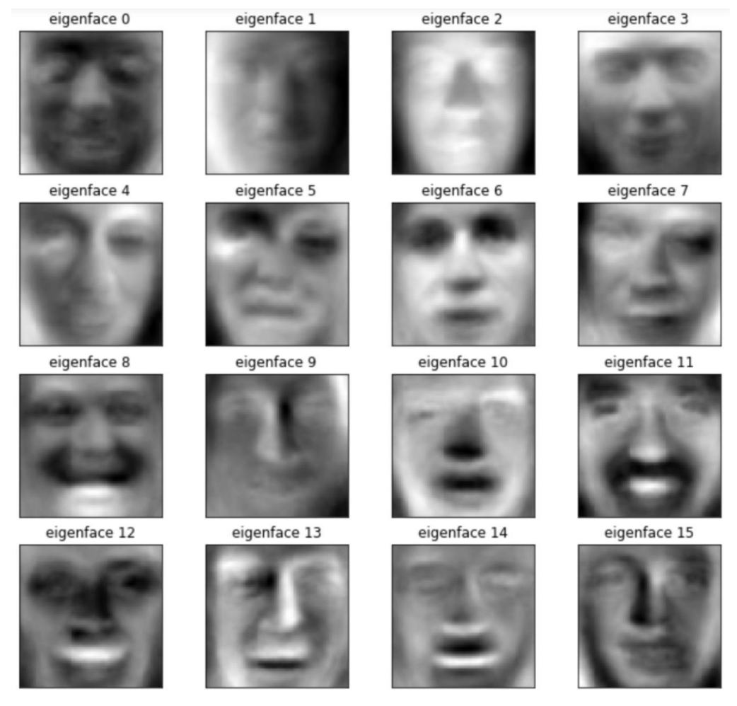
Here's the result of applying PCA on a dataset of faces.

§ Autoencoders

All of these methods discussed so far are precursors of autoencoders.

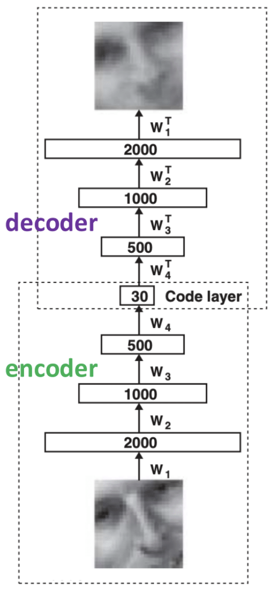
Definition. An autoencoder is any representation that learns its encoder and decoder via deep neural networks (optimized using backpropagation). Its loss, expectedly, is $\mathcal{L}(D, E) := \sum_{x \in X} \|x - D(E(x))\|^2$.

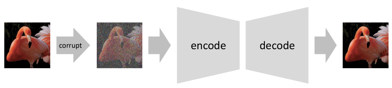
When training an autoencoder, it sometimes helps to corrupt (add noise to) the input data and train the model to recover the clean input. This produces a denoising autoencoder (DAE).

There is also autoencoding with masking (MAE). Here, we train the model to fill in intentionally-masked input.

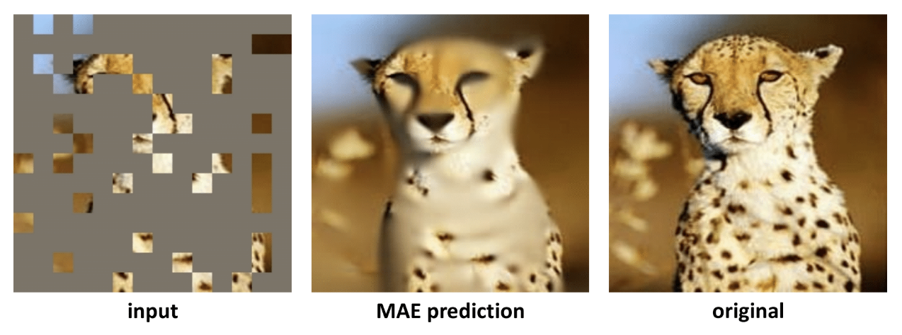
We define the loss to be $\mathcal{L} := \frac{1}{|M|} \sum_{i \in M} \|x_i - \hat{x}_i\|^2$, where $M$ is the set of masked patches, and $\hat{x}_i$ and $x_i$ are the model's guess and the truth, respectively.

§ Similarity-Based Methods: Contrastive Learning

There are many approaches to similarity-based learning—we focus on discussing contrastive learning here.

As a warmup, let's suppose we are in supervised learning, but now equipped with our newly learned encoder.

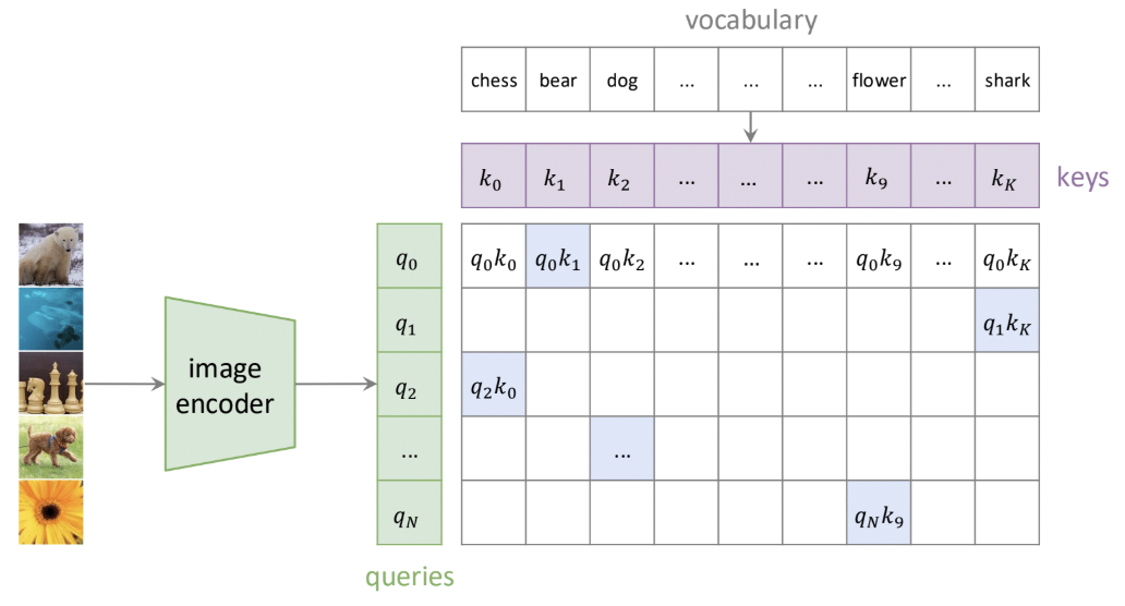
Now that everything is a vector, we might assign a loss by using the dot products $q_ik_j$ like so:

• Penalize dot products that are large when the query and key do not match.

• Penalize dot products that are small when the query and key do match.

We can do this with the loss $\mathcal{L} := -\log \frac{\exp(qk_+)}{\sum_j \exp(qk_j)}$, where $k_+$ is the key matching the query $q$. (This is cross-entropy loss.)

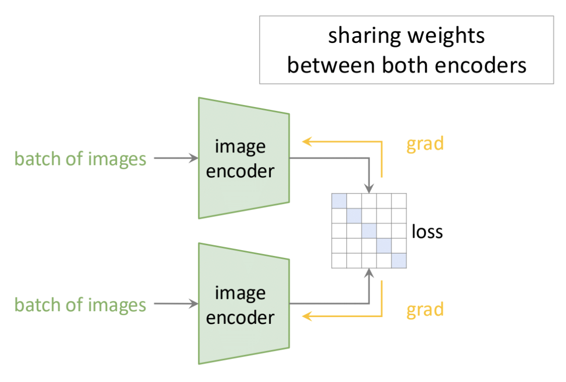
Now for the self-supervised learning case. Instead of taking dot products between image encodings and vocabulary encodings, we can take dot products between encodings of variations of the same image.

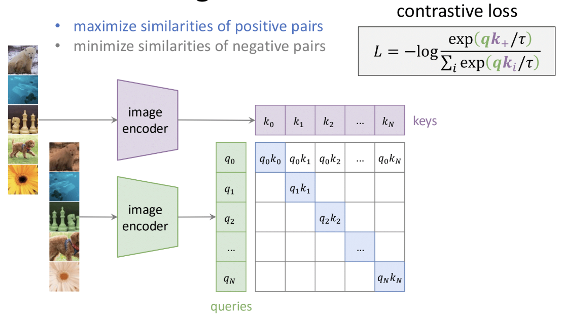
One variation on this is Momentum Contrast (MoCo), where the key encoder is a moving average of the query encoder.

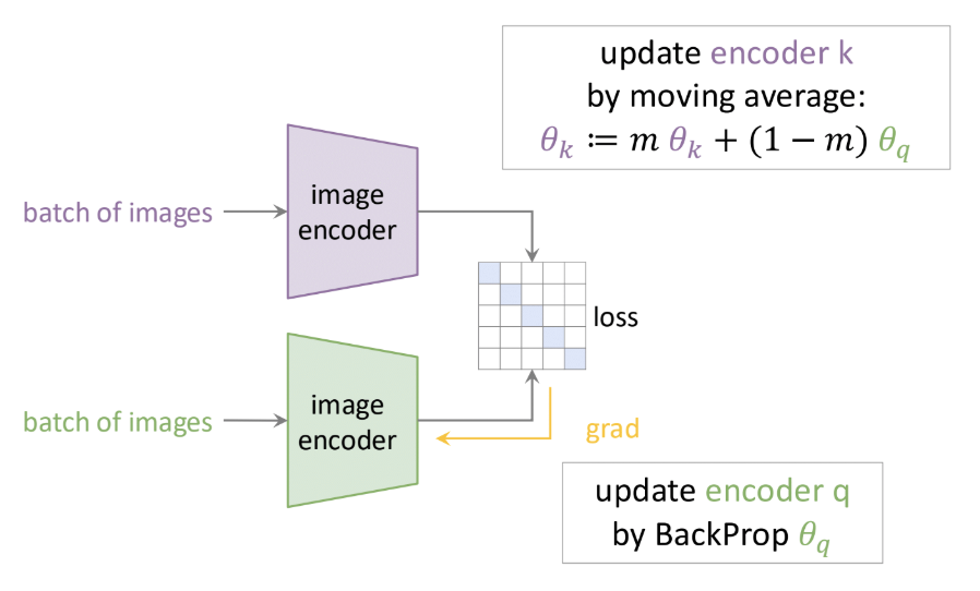
A simpler variation is SimCLR (Simple Framework for Contrastive Learning), where the two encoders share weights.

There are many other similarity-based methods that we won't go over, too.