MIT 6.7960 — Lecture 6

Transformers

§ CNN Limitations

One limitation of CNNs is that they are not well-suited for modeling long-distance relationships.

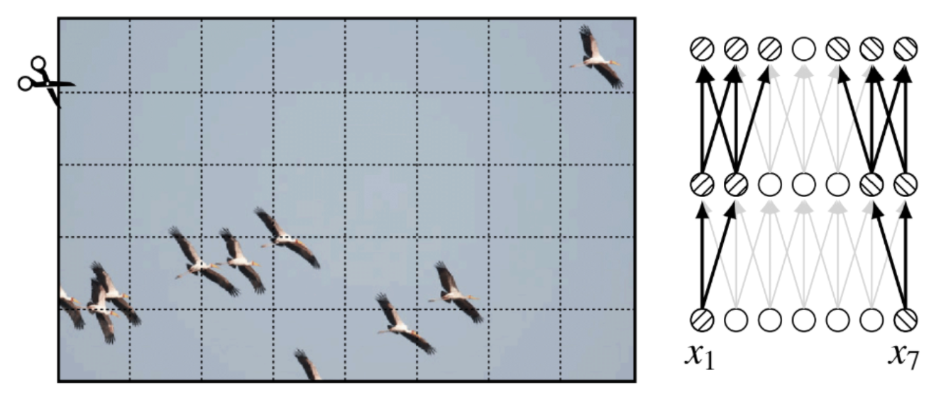Question: How many birds are in this image?

We'll introduce three architectural innovations to fix these problems.

§ Tokens

Definition. A token is just a vector of neurons. Connotatively, a token is an encapsulated bundle of information. You can tokenize anything, whether it's image, text, or audio data.

Here are some details on how tokenization is implemented; the general principle, though is that the details do not matter.

Text is tokenized by using a $\approx$ 100K-entry vocabulary.
- There's usually a pre-tokenization step in which a human-designed regex handles whitespace, punctuation, etc.
- The vocabulary is usually learned separately by simply reading text and identifying common bigrams, trigrams, etc.
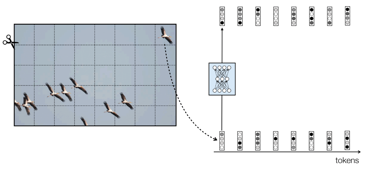
Images are tokenized by simply partitioning the image into patches and vectorizing each patch.
- So a $224 \times 224$ image becomes $196$ vectors if patches of size $16 \times 16$ are used.
- Notably, the tokenization process does not take into account the “content” of the image.
Audio is tokenized by first compressing (e.g., via spectrogram), and only then patching and vectorizing.

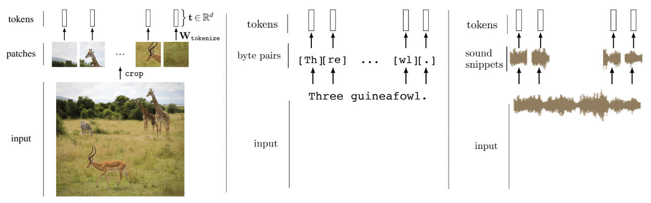
Notably, a very simple tokenization method generally suffices, because the NN on tokens, itself, can learn some of the more interesting relationships between those tokens.

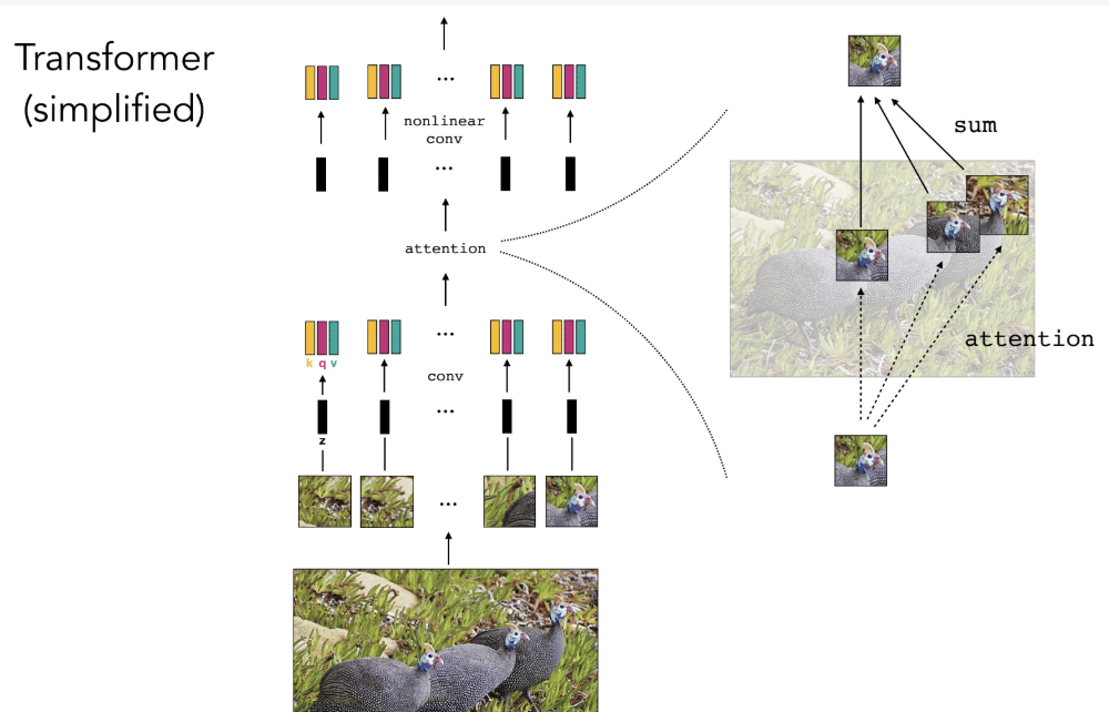
Here's how tokens look when used as nodes in a neural network (at left).

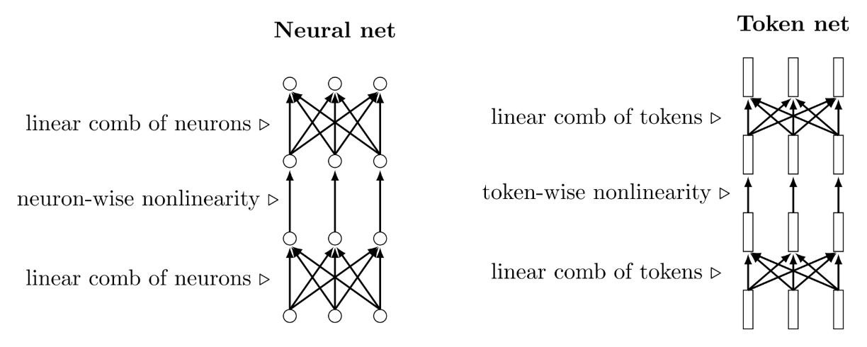
The linear portions of the NN work how you would expect them to.

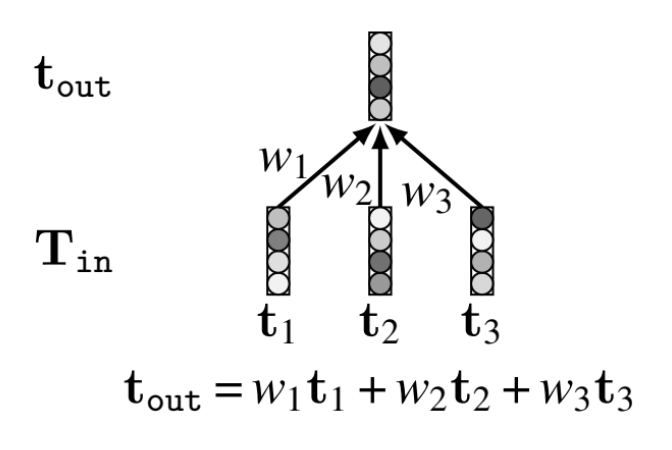
The nonlinear mappings from individual tokens to individual tokens are implemented not with a $\mathrm{ReLU}$ , but with an NN! (Meta.)

§ Query-Key-Value Attention

Currently, the architecture of NN has no way of identifying which tokens are relevant and which tokens are not. We would like our NN architecture to weight our tokens based on how relevant they are to the query.

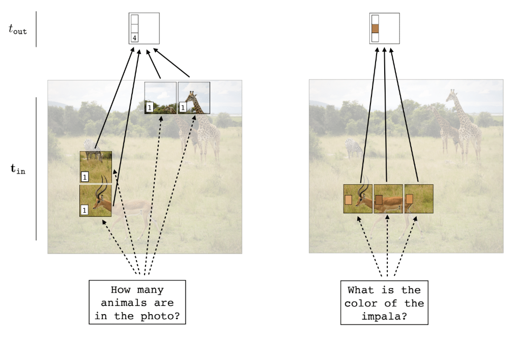
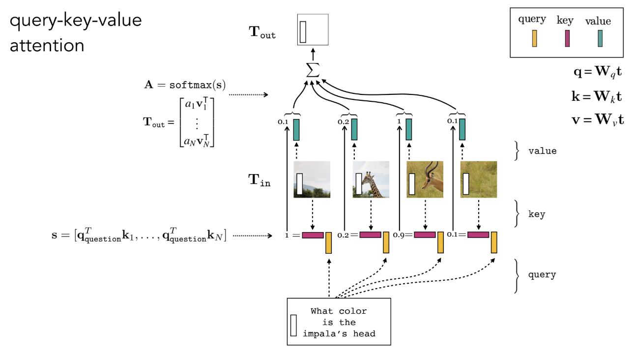
One way to implement this is via query-key-value attention.

Each “input token” $\mathbf{t}$ is mapped to a query token $\mathbf{q} := \mathbf{W}_q\mathbf{t}$ (shown in orange, below).
Each “image token” $\mathbf{t}$ is mapped to a key token $\mathbf{k} := \mathbf{W}_k\mathbf{t}$ (shown in purple, below).
For each pair of image token $\mathbf{a}$ and input token $\mathbf{b}$ , we can determine the relevance of $\mathbf{a}$ and $\mathbf{b}$ by computing the dot product of their query and key tokens $\mathbf{s} = \mathbf{q}_{\mathbf{b}}^{\top} \mathbf{k}_{\mathbf{a}}$ .
Each “image token” $\mathbf{t}$ is mapped to a value token $\mathbf{v} := \mathbf{W}_v \mathbf{t}$ .
- One could simply take $\mathbf{W}_v$ to be the identity; it's just extra expressivity.
The output $\mathbf{T}_{\mathrm{out}}$ is determined by a weighted sum of the values $\{\mathbf{v}\}$ with weights given by the softmax-normalized scores $\mathbf{s}$ .

§ Self-Attention

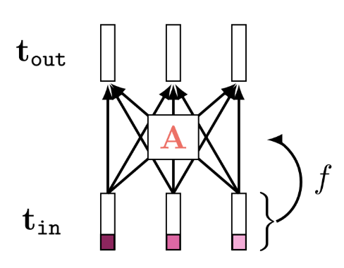
One can also consider self-attention—instead of computing the relevance between input and image, we compute the relevance between some data and itself.

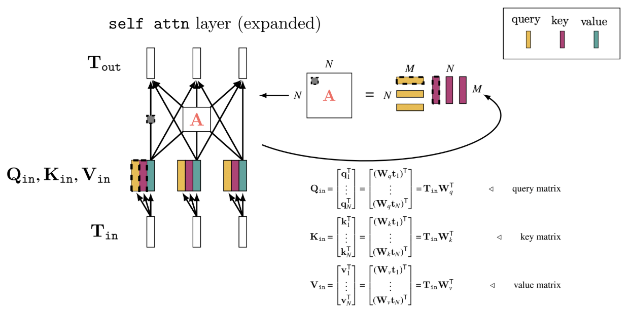
Notably, the map from $\mathbf{T}_{\mathrm{in}}$ to $\mathbf{T}_{\mathrm{out}}$ looks like:

\mathbf{T}_{\mathrm{out}} = \underbrace{\mathrm{softmax}\left( \frac{\mathbf{Q}_{\mathrm{in}}\mathbf{K}_{\mathrm{in}}^{\top}}{\sqrt{m}} \right)}_{\mathbf{A}} \mathbf{V}_{\mathrm{in}}

where $m$ is the query/key dimension. Note that $\mathbf{A}$ is normalized so that each of its rows sum to $1$ , so every output token is a weighted average of all the value tokens; the weight on $\mathbf{v}_j$ in output token $i$ is $\mathbf{A}_{ij} \propto \exp(\mathbf{q}_i^{\top}\mathbf{k}_j / \sqrt{m})$ .

Relevance is measured under the learned maps: $\mathbf{q}_{\mathbf{a}}^{\top}\mathbf{k}_{\mathbf{b}} = \mathbf{a}^{\top}\mathbf{W}_q^{\top}\mathbf{W}_k\mathbf{b}$ , which is not symmetric.
- So “A attends to B” is distinct from “B attends to A” (and neither are exactly equivalent to “A and B are similar”).
Unlike in CNNs, every pair of tokens is connected by a single matrix multiplication, no matter how far apart they are.

Below, the learned projections happen to make each bird-head patch attend to the other bird-head patches.

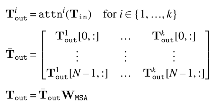
Definition. There's also multihead self-attention (MSA), in which we concatenate $k$ different attempts at self-attention tokenwise, then project back down with a matrix $\mathbf{W}_{\mathtt{MSA}}$ .

§ Transformer Architecture

Putting together multihead self-attention (MSA) with multi-layer perceptrons (MLPs), we get a transformer!

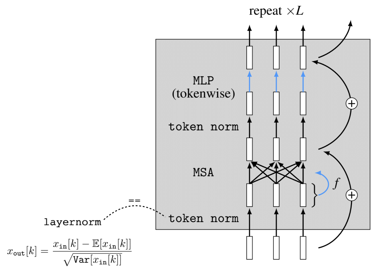
The code for a transformer is extremely simple, too.

# x: input data (RGB image)
# K: tokenization patch size
# d: token/query/key/value dimensionality (setting these all as the same)
# L : number of layers
# W_q_T, W_k_T, W_v_T : transposed query/key/value projection matrices
# mlp: tokenwise mlps

# tokenize input image
T = tokenize(x, K) # 3 x Hx W image --> N xd array of token code vectors

# run tokens through all L layers
for l in range(L):

    # attention layer
    Q, K, V = nn.matmul(nn.layernorm(T), [W_q_T[l], W_k_T[l], W_v_T[l]])
    # nn.matmul does matrix multiplication
    A = nn.softmax(nn.matmul(Q,K.transpose())/sqrt(d), dim=-1)
    T = nn.matmul(A, V) + T # note residual connection

    # tokenwise mlp
    T = mlp[l](nn.layernorm(T)) + T # note residual connection

# T now contains the output token representation computed by the transformer

§ Positional Encodings

One observation about the transformer architecture is that it is permutation equivariant.

F_{\theta}(\pi(\mathbf{T}_{\mathrm{in}})) = \pi(F_{\theta}(\mathbf{T}_{\mathrm{in}})) ~~~ \text{ and } ~~~ \textsc{attn}(\pi(\mathbf{T}_{\mathrm{in}})) = \pi(\textsc{attn}(\mathbf{T}_{\mathrm{in}})) ~~~ \text{ for any MLP } F_{\theta} ~ \text{ and any MSA } \textsc{attn}.

But we actually don't want permutation equivariance, because that implies that it may be difficult for models to learn about forms of data that care about position. The fix, naturally, is to add position to each of our tokens.

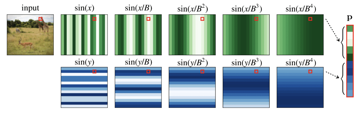
There is some nuance concerning how, exactly, we encode position. For images, for example, we might encode position by the Fourier coefficients associated with that position.

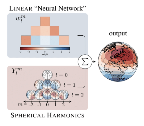
Similarly, positional encodings of points on a sphere might use spherical harmonics.

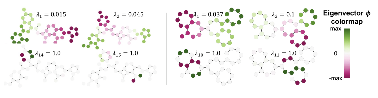
Positional encodings of nodes in a graph are given by the eigenvectors of its Laplacian. (Details omitted.)

§ Autoregressive Models (GPT, Claude)

Recall that LLMs like GPT generate text by “predicting the next word”.

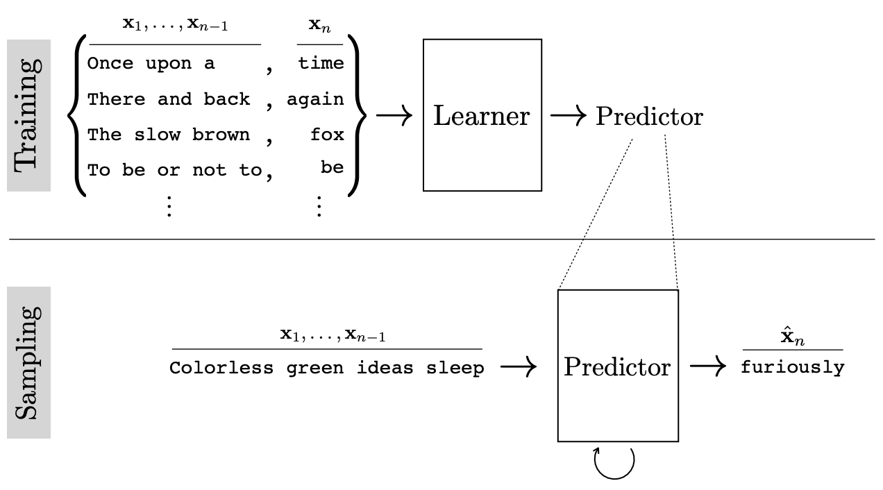
GPT's means of prediction is basically just a transformer. The only distinction is that the attention matrix must forbid some tokens attending to tokens that occur in the future. To implement this, it suffices to mask $\mathbf{A}$ like so:

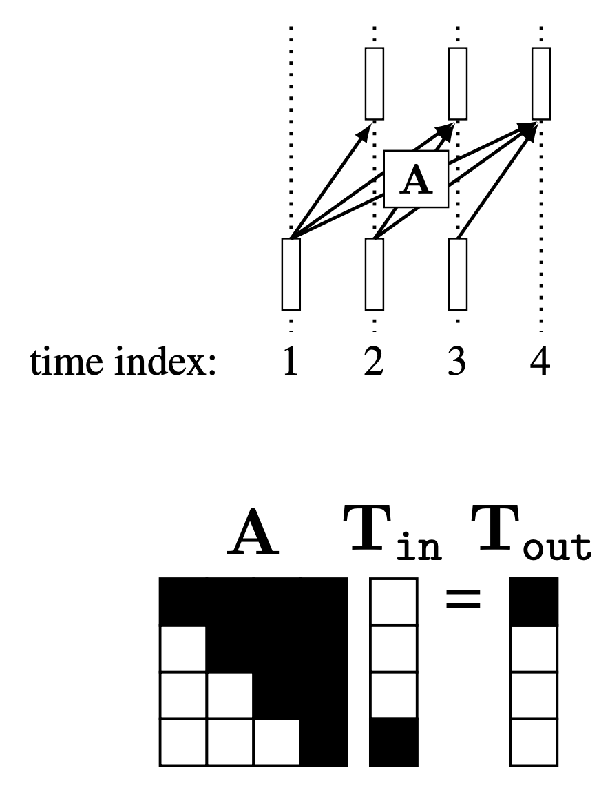
More generally, here's how the causal self-attention relationships look for autoregressive image-to-text architectures.

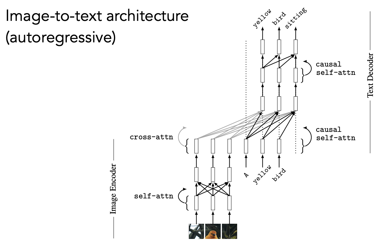
We call this cross-modality attention, because attention occurs between data in both text and image modalities.