MIT 6.4210 — Lecture 3

Frames, Monogram Notation, and Rotations

§ Frames

Note that $\mathbb{E}^3$ denotes an affine space. Informally, it's $\mathbb{R}^3$ without an origin—so it has subtraction and distances, but no addition. In robotics, we work in $\mathbb{E}^3$ instead of $\mathbb{R}^3$ because we oftentimes can't pick a single universally-meaningful origin.

Definition. In robotics, a frame (similar to a basis in linear algebra) describes a frame of reference using the following data.

\text{frame} ~ = ~ (\text{origin } O \in \mathbb{E}^3, ~ \text{basis } (\hat{x}, \hat{y}, \hat{z})), ~~~ \text{ where } (\hat{x}, \hat{y}, \hat{z}) \text{ must be orthonormal and right-handed.}

Note that every body $i$ has a frame $B_i$ associated with it. (Imagine an airplane, for example.)

Definition. Drake has a built-in world frame denoted $W$ .

Definition. Any frame is defined by its position $O$ and its orientation $(\hat{x}, \hat{y}, \hat{z})$ . This data is collectively called spatial pose.

When we refer to “the pose of an object $O$ ”, we really mean “the pose of the body frame of $O$ in the world frame $W$ ”.

§ Monogram Notation

Definition. We write $^B p^A_C$ to denote the vector $\vec{BA}$ expressed in frame $C$ . (So $^B p^A_C$ is a tuple of $3$ real numbers.) Furthermore,

Since all frames $F$ have a position, it is valid to write something like $^{F_1}p^{F_2}_{F_3}$ .
For any frame $F$ , the notation $^Fp^A$ is shorthand for $^Fp^A_F$ .
For a point $B$ that isn't a frame, $^Bp^A$ is shorthand for $^Bp^A_W$ .

Definition. For any two frames $F$ and $G$ , we say:

The notation $^FR^G$ denotes the rotation that sends the orientation of $F$ to the orientation of $G$ .
The notation $^FX^G$ denotes the spatial transform that sends the spatial pose of $F$ to the spatial pose of $G$ .

Definition. The Drake documentation suggests the following variable names:

^Bp^A_C = \verb|p_BA_C| ~~~~~~~~~ ^FR^G = \verb|R_FG| ~~~~~~~~~ ^FX^G = \verb|X_FG|

Theorem. (Monogram Algebra) The following identities are all true.

{}^Ap^B_F + {}^Bp^C_F = {}^Ap^C_F ~~~ \parallel ~~~ {}^Ap^B_F = - {}^Bp^A_F ~~~ \parallel ~~~ {}^Ap^B_G = {}^GR^F {}^Ap^B_F ~~~ \parallel ~~~ {}^AR^B {}^BR^C = {}^AR^C

Proof: The first, second, and fourth of these are obvious. The third is surprisingly unintuitive—think through it carefully. $\blacksquare$

Remark. There are two ways to think about the rotation $^AR^B$ .

It is a map from the orientation of $A$ to the orientation of $B$ .
It is a map that, for any point $Q$ , sends the coordinates of $Q$ in the frame of $B$ to the coordinates of $Q$ in the frame of $A$ .

We now dedicate the rest of this lecture to giving examples of how we actually describe rotations numerically.

§ Rotation Matrices

Just a matrix $M \in SO_3(\mathbb{R})$ . The main nontrivial point to be aware of is that $M^{-1}$ is very easy to compute—it's just $M^{-1} = M^{\top}$ .

Note, also, that using $9$ numbers for a data structure that describes rotation in $\mathbb{R}^3$ is, in some sense, wasteful. There are ways to describe rotations using fewer than $9$ numbers, such as…

§ Roll, Pitch, Yaw (Euler Angles)

Definition. Let $R_x(\theta)$ denote the rotation about the world's $x$ -axis by $\theta$ . Define $R_y(\theta)$ and $R_z(\theta)$ similarly.

Remark. Use the right-hand rule. If you point your thumb in the direction of the positive $x$ -axis, then your fingers curl in the direction of positive rotations $\theta$ .

Definition. Let $(r, p, y)$ in roll-pitch-yaw denote the rotation $R_z(y)R_y(p)R_x(r)$ (read from right-to-left, as with matrix multiplication). These are also called Euler angles.

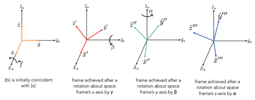
Example. The rotation with roll $90^{\circ}$ , pitch $0^{\circ}$ , and yaw $90^{\circ}$ has the effect of permuting the axes $(x, y, z) \mapsto (y, z, x)$ .

Theorem. (Extrinsic vs. Intrinsic) Given rotation angles $(r, p, y)$ and an object $O$ , consider the following rotations on $O$ , where the extrinsic axes are the world's axes, whereas the intrinsic axes are the basis of the frame of $O$ .

Rotate by $r$ about the extrinsic $x$ -axis, then rotate by $p$ about the extrinsic $y$ -axis, then rotate by $y$ about the extrinsic $z$ -axis.
Rotate by $y$ about the intrinsic $z$ -axis, then rotate by $p$ about the intrinsic $y$ -axis, then rotate by $r$ about the intrinsic $x$ -axis.

Then these two rotations are the same.

Proof: Say the rotations about the extrinsic axes have rotation matrices $R_X$ , $R_Y$ , and $R_Z$ . Then the intrinsic rotations are…

“rotate by $y$ about the intrinsic $z$ -axis” $\implies$ this is equivalent to $R_Z$ .
“then rotate by $p$ about the intrinsic $y$ -axis” $\implies$ this is equivalent to $R_ZR_YR_Z^{-1}$ …
- … because it's equivalent to “undo the previous rotation, then apply $R_Y$ , then redo the previous rotation”.
“then rotate by $r$ about the intrinsic $x$ -axis” $\implies$ this is equivalent to $(R_ZR_YR_Z^{-1}R_Z)R_X(R_ZR_YR_Z^{-1}R_Z)^{-1}$ …
- … for the same reason as the previous bullet.

And composing all three gives $(R_ZR_Y)R_X(R_ZR_Y)^{-1} \cdot R_ZR_YR_Z^{-1} \cdot R_Z = R_ZR_YR_X$ , as desired. $\blacksquare$

The problem with using Euler angles to parametrize the space of rotations is that this parametrization produces gimbal lock.

Example. Consider the subspace of roll-pitch-yaw rotations $\{(r, 90^{\circ}, y) \mid r, y \in \mathbb{R}\}$ . This happens to be a one-dimensional subspace, despite there being $2$ free parameters $(r, y)$ .

The following (warning: AI-generated) widget gives a visual demonstration of gimbal lock when $p = 90^{\circ}$ .

Remark. The “only” times when gimbal lock occurs are when $p = \pm 90^{\circ}$ —you should intuitively be able to see why using the widget above. (What is the only way that two axes can overlap with each other?)

In fact, it has been proven (Stuelpnagel, 1964) that no parametrization of $SO_3(\mathbb{R})$ with three variables can avoid gimbal lock.

§ Axis-Angle

Recall from 18.701 that every rotation in $SO_3(\mathbb{R})$ looks like a rotation about some axis $\hat{v}$ through the origin by some angle $\theta$ . So one natural way to encode a rotation is through the three-variable vector $\theta \cdot \frac{\hat{v}}{\|\hat{v}\|}$ .

Of course, this parametrization also produces gimbal lock, because it has exactly three variables.

§ Quaternions

See 18.701 for a more rigorous discussion of the quaternions $\mathbb{H}$ (along with the group of unit quaternions $SU_2$ ). Here's the main point we need to know.

Theorem. (Unit Quaternions as Rotations) The unit quaternion $(w, x, y, z) \in SU_2$ represents a rotation about axis $\hat{v}$ by angle $\theta$ (with $\|\hat{v}\| = 1$ ) if we have $w = \cos\left(\frac{\theta}{2}\right)$ and $\left[\begin{smallmatrix} x \\ y \\ z \end{smallmatrix}\right] = \sin\left(\frac{\theta}{2}\right) \hat{v}$ .

Example. A rotation by $\theta = 60^{\circ}$ about the axis $\hat{v} = \left[\begin{smallmatrix} 2/3 \\ 2/3 \\ 1/3 \end{smallmatrix}\right]$ can be expressed by the quaternion $\left(\frac{\sqrt{3}}{2}, \frac{1}{3}, \frac{1}{3}, \frac{1}{6}\right)$ .