MIT 6.4210 — Lecture 5

Inverse Kinematics via Optimization

§ Inversion as Optimization: Constraints

Recall from Lecture 4 that our approach to solving “inverse” problems is to take the (damped, possibly) pseudo-inverse, because it nicely satisfies the following properties.

Theorem. (Pseudo-Inverse Approximation) For any matrix $J$ and vector $b$ (with appropriate dimensions), the vector $x^* := J^+b$ is the vector with minimum magnitude across all vectors that minimize $\|Jx - b\|$ . In particular,

If the column space of $J$ does not contain $b$ , then $x^* := J^+b$ is such that $\|Jx - b\|$ is minimized.
If the column space of $J$ contains $b$ (that is, $\|Jx - b\|$ can be zero), then $x^* := J^+b$ is the solution to $Jx = b$ minimizing $\|x\|$ .

We can go even further, though, by phrasing this as an optimization problem.

Quadratic Program. Find the vector $x^*$ with minimum magnitude that minimizes $\|Jx^* - b\|^2$ .

Viewing this as a quadratic program (see 6.1220 Notes for context), we can also consider adding constraints to this problem. For example, we might want to specify that $|\mathrm{d}q_1| \leq 10$ , $|\mathrm{d}q_2| \leq 10$ and $\mathrm{d}q_1^2 + \mathrm{d}q_2^2 \leq 150$ to prevent exploding velocities.

Notice that this is not just as simple as taking the output of the pseudo-inverse and clipping it to a constrained region!

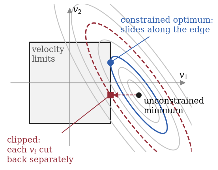
As the image above indicates, the solution achieved by clipping (shown in red) can oftentimes be less optimal than the solution achieved by optimizing the constrained quadratic program (shown in blue).

§ Inversion as Optimization: Joint Centering

Now suppose that our system is highly redundant—there are infinitely many $\mathrm{d}q$ that achieve $J(q) \mathrm{d}q = \mathrm{d}X^B$ . Can we get something out of the fact that our null space is nontrivial?

Well, the pseudo-inverse exploits this by specifically aiming for the solution $\mathrm{d}q$ with smallest magnitude.

But maybe, more smartly, we can specify a preferred position $q^d$ . Then if our current state is $q$ , we might imagine a spring of stiffness $K$ that induces a desired velocity of $K(q^d - q)$ .

Since the null space is nontrivial, we can project this desired velocity $K(q^d - q)$ into the null space. This lets us freely add the projection into $\mathrm{d}q$ without affecting the fact that $J(q) \mathrm{d}q = \mathrm{d}X^B$ . See the (warning: AI-generated) widget below.

This is fairly widely used, especially for robots that are highly redundant.

§ Trajectory Optimization

A common constraint that one might use is that the robot must avoid collisions. In the very simple example of a 2D simplified two-rod Kuka IIWA, here's how that constraint looks in the configuration space $(q_1, q_2)$ .

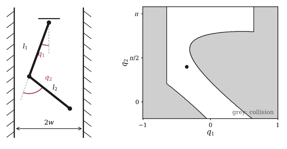
Notably, this constraint is non-convex, so it cannot simply be solved by traditional quadratic program solvers. (For example, gradient descent can get stuck in a local minimum.)

One might define a trajectory optimization problem like so:

Trajectory Optimization. Minimize $\sum_{n = 0}^{N - 1} \| q[n + 1] - q[n] \|^2$ such that $q[0] = q_{\mathrm{start}}$ , $q[N] = q_{\mathrm{goal}}$ , and the path $q[0] \to q[1] \to \dots \to q[N]$ does not collide with anything.

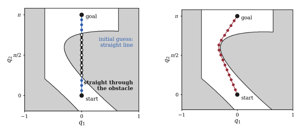
An optimizer might then start with an initial guess and gradually improve the guess, in hopes that the local minimum that it converges towards does actually satisfy the nonconvex constraints.

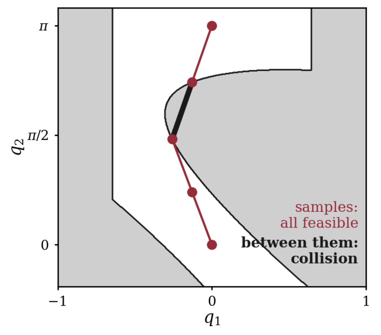
Given a set of points $\{q[n]\}_{n = 0}^N$ , we can define a path via a B-spline, for example.

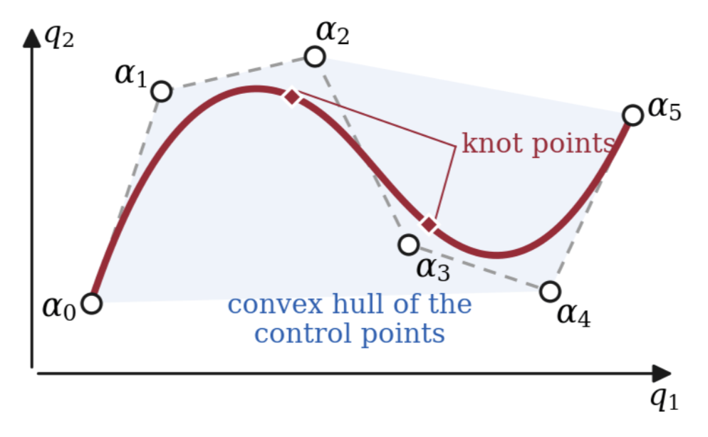
One nice property of B-splines is that the curve always stays within the convex hull of the control points. But one bad property of B-splines is that even if the control points satisfy the constraints, the path itself might not.

Next lecture, we'll discuss alternative (non-optimization-based) approaches to motion planning.