MIT 6.4210 — Lecture 6

§ Motion Planning: Setup

Definition. Some reminders of some definitions:

• The work space (or Cartesian space) of a robot is the set of points reachable by an end-effector.

  • For example, one might use $(x, y, \theta)$ to parametrize the work space of a two-rod 2D Kuka IIWA.

• The configuration space of a robot is the set of reachable configurations of the robot—not just the end-effector!

  • A configuration is denoted $\mathbf{q} \in C$, where $C$ is the set of all possible configurations.

  • For example, one might use $(q_1, q_2)$ to parametrize the configuration space of a two-rod 2D Kuka IIWA.

    • The topology of the configuration space might not be Cartesian; in this example, it's $S^1 \times S^1$ (a torus).

Definition. In motion planning, we assume that we have:

• A world $W$.

• An obstacle region $O \subset W$.

• A robot $A$ defined in $W$ (i.e., $A \subset W$).

• We seek a collision-free path from $\mathbf{q}_I \in C$ to $\mathbf{q}_G \in C$.

§ Motion Planning: Obstacle Space

Given a robot $A$ and an object $O$, how can we determine the set of positions of $A$ in which $A$ and $O$ do not intersect?

Definition. We define the obstacle space $C_{\mathrm{obs}} \subset C$ by $C_{\mathrm{obs}} := \{q \in C \mid A(q) \cap O \neq \emptyset\}$, in addition to $C_{\mathrm{free}} = C \setminus C_{\mathrm{obs}}$.

In simple translational cases, we can write $C_{\mathrm{obs}} = O \ominus A$, where $\ominus$ is the Minkowski difference.

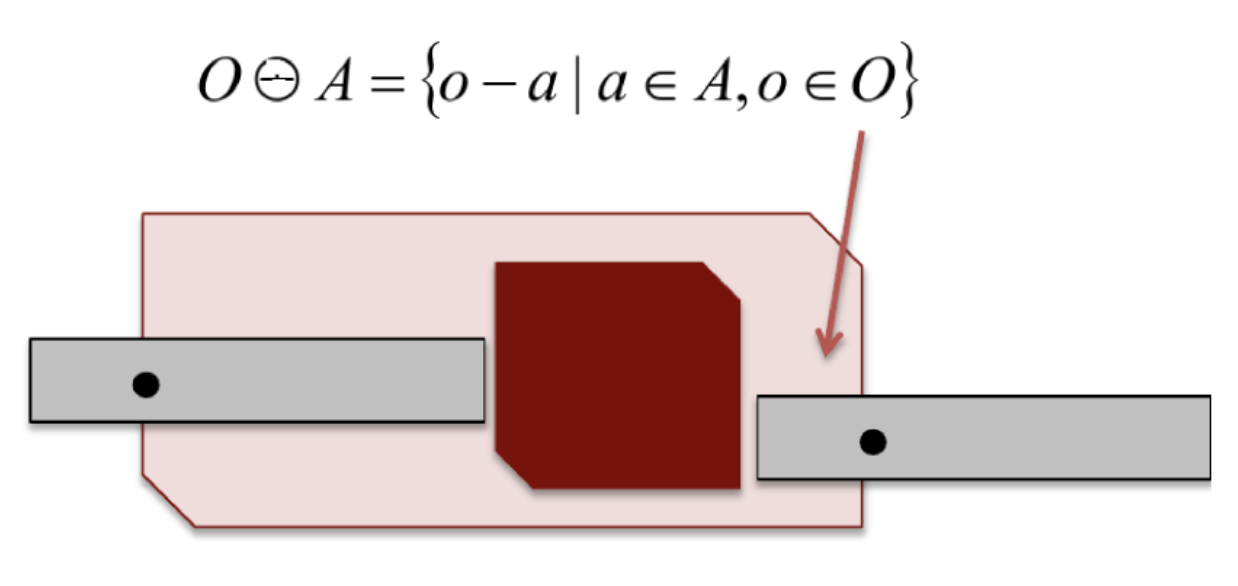
The Minkowski difference can be efficiently computed using the Star algorithm—details omitted.

But for nontranslational cases, the obstacle space can be harder to compute. For example, the robot might be allowed to rotate, or the configuration space might be non-Cartesian.

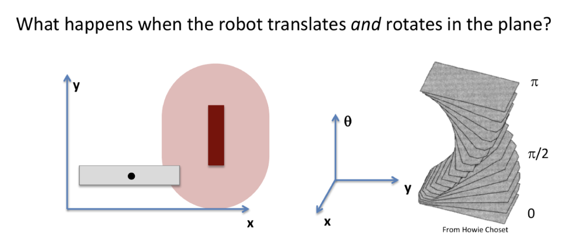
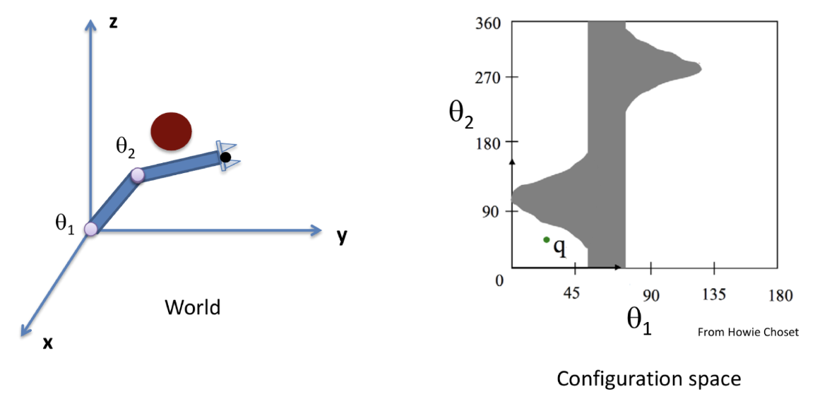
In some of these cases, the runtime for computing $C_{\mathrm{obs}}$ might be exponential!

The upshot of defining $C_{\mathrm{obs}}$ is that we can now define the problem of motion planning entirely within the configuration space $C$.

Definition. In motion planning, we assume that we have:

• A configuration space $C$, plus an obstacle space $C_{\mathrm{obs}} \subset C$ and a free space $C_{\mathrm{free}} := C \setminus C_{\mathrm{obs}}$.

• We seek a continuous path $\tau \colon [0, 1] \to C_{\mathrm{free}}$ with $\tau(0) = \mathbf{q}_I$ and $\tau(1) = \mathbf{q}_G$.

§ Combinatorial Planning

Definition. A motion planner is complete if it always finds a solution if one exists and returns a failure in bounded time if not.

The combinatorial algorithms we discuss in this section will be complete, and they will all employ road maps.

Definition. Given a configuration space $C$ and a free space $C_{\mathrm{free}}$, a road map $R$ is a graph whose vertices are configurations in $C_{\mathrm{free}}$ and whose edges are collision-free paths between vertices. This graph must be such that:

• (Accessibility) For any starting point $q_I \in C_{\mathrm{free}}$, it is easy to find a collision-free path $q_I \to q'$ for some $q' \in R$.

• (Departability) For any ending point $q_G \in C_{\mathrm{free}}$, it is easy to find a collision-free path $q' \to q_G$ for some $q' \in R$.

• (Connectivity) If $q_1, q_2 \in R$ are connected in $C_{\mathrm{free}}$, then they are connected in the graph of $R$.

Here's an example of how a road map might let us find a collision-free path $q_I \to q_G$.

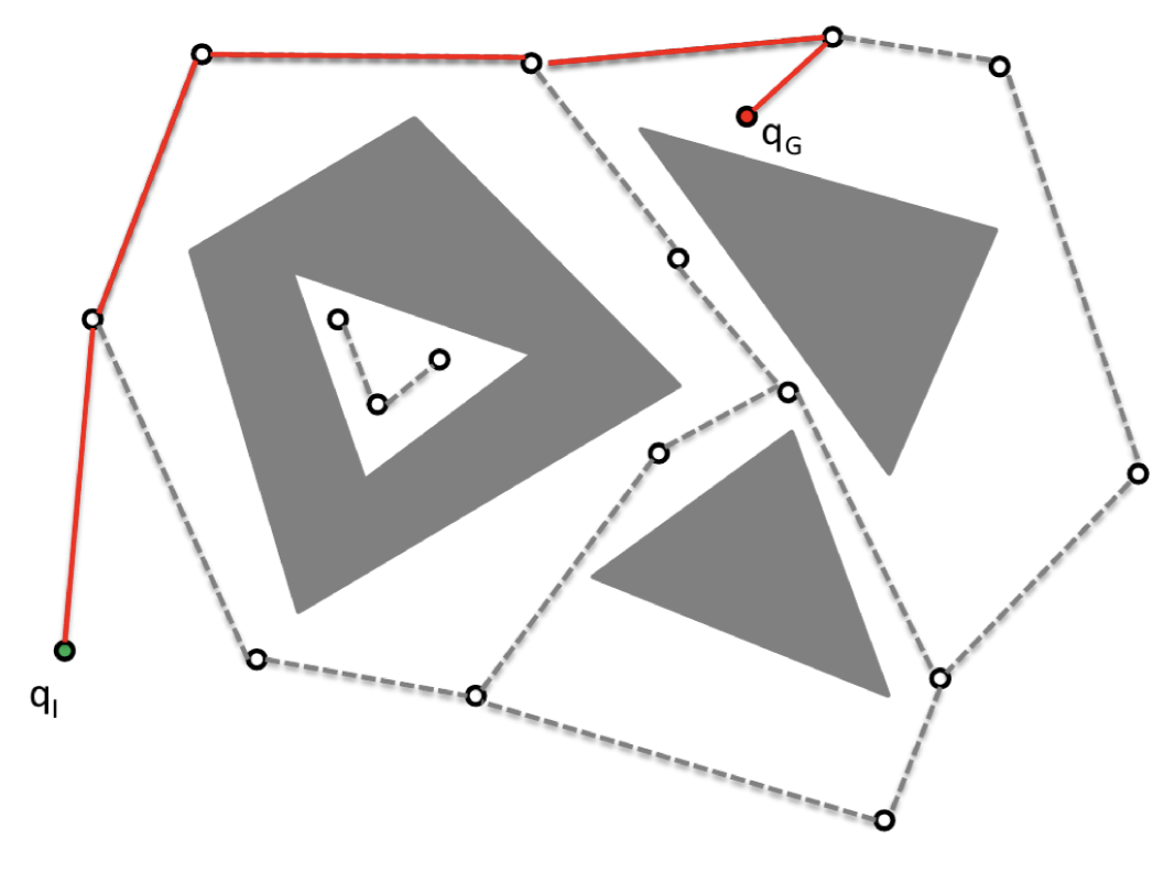
Here are some different strategies for constructing road maps.

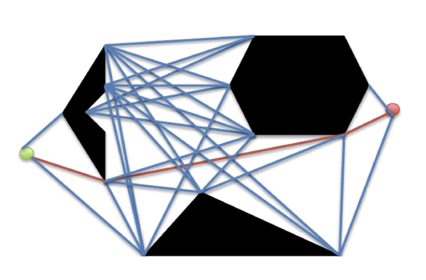
Visibility Graph. Suppose the configuration space is $\mathbb{R}^2$, and every obstacle is a convex polygon. (If an obstacle is concave, you can work around this by breaking it up into convex pieces.)

Then for any $q_I, q_G \in C_{\mathrm{free}}$, to find a path $q_I \to q_G$, we simply:

• Precompute for any two vertices of two polygons, whether the straight-line path between them is collision-free.

• Determine the set of all polygon vertices $q$ for which $q_I \to q$ is collision-free (and separately for $q \to q_G$, too).

• Apply a shortest-path $O(n^2 \log n)$ algorithm (e.g., A*) to find the shortest collision-free path $q_I \to q_G$.

It turns out that this algorithm in fact always finds the shortest collision-free path $q_I \to q_G$.

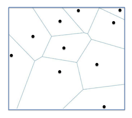
Voronoi Diagram. Just construct the Voronoi Diagram of the obstacles.

The roadmap graph is then exactly the “boundaries” of the Voronoi diagram. In a sense, this lets you keep a maximum distance away from any obstacle throughout your collision-free path.

One last algorithm archetype.

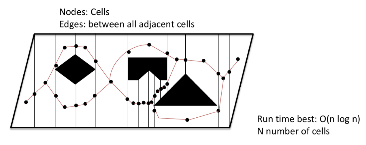
Cell Decomposition. Split the configuration space into cells, and then find paths between the cells.

For example, here's a cell decomposition by $x$-coordinate of the obstacles.

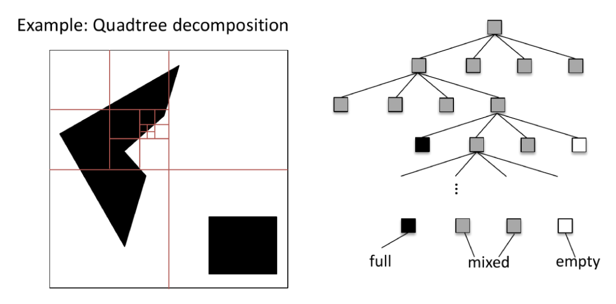
There are also approximate cell decomposition approaches; for example, here's a quadtree decomposition approach.

The idea is that cells are either empty, full, or mixed, and that “mixed” cells can be zoomed into as needed.

As mentioned earlier, these are all complete algorithms (approximate cell decompositions only up to resolution). But their disadvantages are that they become intractable as the obstacle complexity or dimensionality of the $C$-space increases. (And this happens very often in robotic manipulation!)

§ Sampling-Based Planning

Definition. A (randomized) motion planner is probabilistically complete if, assuming a solution exists, the probability of finding that solution in $t$ time tends to one as $t \to \infty$.

The sampling-based algorithms we discuss in this section will be probabilistically complete. There are two kinds:

• Multi-query: The algorithm performs some precomputation—assumes obstacles are fixed across queries.

• Single-query: The algorithm does not perform precomputation—useful when obstacles move over time.

Here's the most common multi-query algorithm.

Probabilistic Roadmap (PRM). Construct the roadmap $R = (V, E)$ procedurally by repeating the following algorithm.

1. Randomly pick a point $q \in C$ and check if $q \in C_{\mathrm{free}}$. If it isn't, try again.

2. If it is, add $q$ to $V$, and for each $q' \in V$ with $\|q - q'\| < d$, add the edge $q \leftrightarrow q'$ to $E$ if that path is collision-free.

The whole point of PRM is to avoid having to compute $C_{\mathrm{obs}}$. Instead, for each $q \in C$, it uses a custom collision-detector to check whether $q \in C_{\mathrm{free}}$. (Efficient collision-detectors exist, because video games require them.)

As shown above, though, the paths outputted by PRM are not very short. Here are some improvements to PRM:

• Find shortcuts—between two points on the path, ask if the straight line between them is collision-free.

  

• Use paths generated by PRM as starting paths for the optimization algorithms described in Lecture 5.

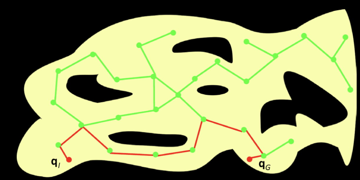
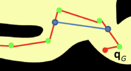
Unfortunately, PRM may fail with nonzero probability because the roadmaps it produces might not satisfy Accessibility and Departability or Connectivity, as shown below.

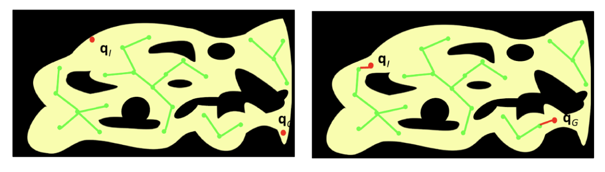
But PRM just works very well in practice because—even in high dimensions—collision-detection is still very fast.

Sometimes the obstacles do move around, though, in which case we require single-query algorithms.

Rapidly-Exploring Random Trees (RRT). We gradually add points to a connected tree in the following way.

1. Randomly pick a point $q_{\mathrm{rand}} \in C$ and check if $q_{\mathrm{rand}} \in C_{\mathrm{free}}$. If it isn't, try again.

   • With probability $p$ (the goal bias), our random point $q_{\mathrm{rand}}$ will just be $q_{\mathrm{rand}} = q_G$, the goal.

2. (Extend) If it is, then do the following:

   • Find the nearest point $q' \in T$ to $q_{\mathrm{rand}}$.

   • Compute the point $q_{\mathrm{new}}$ that is $\eta$ of the way between $q'$ and $q_{\mathrm{rand}}$, for some fixed constant $\eta \in (0, 1)$.

   • If the segment $q' \to q_{\mathrm{new}}$ lies in $C_{\mathrm{free}}$, then append $q_{\mathrm{new}}$ to $T$ and connect $q'$ and $q_{\mathrm{new}}$ with a collision-free path.

You can see this algorithm in action using the (warning: AI-generated) widget below.

RRT RRT-Connect RRT*

Walls Clutter Passage

Step Run Reset

q_I (drag) q_G (drag) q_rand q_new

Step η

0.50

Goal bias

5%

Note that this algorithm is not the same as a plain random walk—a random walk doesn't tend to go anywhere, whereas RRT will eventually tend to fill the space.

A natural speed-up is RRT-Connect, in which we grow a tree from both $q_I$ and $q_G$ bidirectionally.

1. Grow trees $T_A$ and $T_B$ out of $q_I$ and $q_G$, respectively.

2. Suppose RRT adds a new vertex $q_{\mathrm{new}}$ to $T_A$ (Extend). Then:

   • Take the nearest point $q' \in T_B$ to $q_{\mathrm{new}}$ and take steps (Extend) from $q'$ to $q_{\mathrm{new}}$ until a collision occurs.

   • Add any taken steps to the tree $T_B$. Then swap $T_A$ and $T_B$.

     • Allegedly, taking $T_A$ to always be the smaller tree helps even more.

3. Repeat until the steps taken from $q'$ to $q_{\mathrm{new}}$ reach $q_{\mathrm{new}}$ without any collisions.

You can see in the widget above that RRT-Connect is much better than RRT for navigating narrow passages.

One last improvement is RRT*, which favors shorter paths between $q_I$ and $q_G$. Handwavily, it adapts RRT in two ways:

• Connect each $q_{\mathrm{new}}$ to whichever nearby $q' \in T$ gives the shortest path from $q_I$—not necessarily the $q'$ closest to $q_{\mathrm{new}}$.

• Afterwards, rewire $T$: if a nearby $q' \in T$ would have a shorter path from $q_I$ through $q_{\mathrm{new}}$, reroute it through $q_{\mathrm{new}}$.

RRT* keeps running even after it reaches $q_G$ so that even shorter paths can be found over time.

One advantage of RRT is that it works even for non-holonomic robots.

Definition. A robot is holonomic if it can freely move in any direction in its configuration space.

• The simplified 2D two-rod Kuka IIWA is a holonomic robot.

• A car is not a holonomic robot; it cannot translate its body in a lateral direction.

Combinatorial planning algorithms ask whether you can move from $q_1$ to $q_2$ in the configuration space, which is not easily answerable for non-holonomic robots.

But RRT only asks whether, starting from $q'$, you can get closer to $q_{\mathrm{rand}}$, thereby landing on $q_{\mathrm{new}}$. This can be answered for non-holonomic robots by forward-simulating various inputs and checking whether any results land closer to $q_{\mathrm{rand}}$.

Spoilers: it turns out that RRT (or variants of it) just perform the best in practice.