MIT 6.4210 — Lecture 4

Basic Kinematics

§ Task vs. Configuration Space

Recall the distinction between task space and configuration space. For example, given a Kuka IIWA manipulator…

The task space consists of just the position, orientation, and velocity of its end effector.
The configuration space is much larger—it consists of all the angles and velocities at all $7$ of its joints.

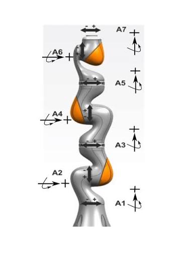
Last lecture, we discussed how we represent and work with the task space of the end effector. In this lecture, we work in the configuration space—how should we move the joints such that the gripper moves to the state we desire?

Definition. We often talk about the following forms of kinematics.

Forward Kinematics: Given the joint positions, what is the end effector pose?
Inverse Kinematics: Given the final pose, what are the joint positions?
Differential Kinematics: Given the joint positions and velocities, what is the end effector pose and velocity?
Differential Inverse Kinematics: Given the end effector pose and velocity, what are the joint positions and velocities?

§ Forward Kinematics

As one might expect, forward kinematics is purely deterministic and very easy to compute: just compose transforms. To demonstrate, here's how that looks for a simplified 2D Kuka IIWA.

{}^aX^2(q_0, q_1) = {}^aX^0 \ {}^0X^b(q_0) \ {}^bX^1 \ {}^1X^c(q_1) \ {}^cX^2

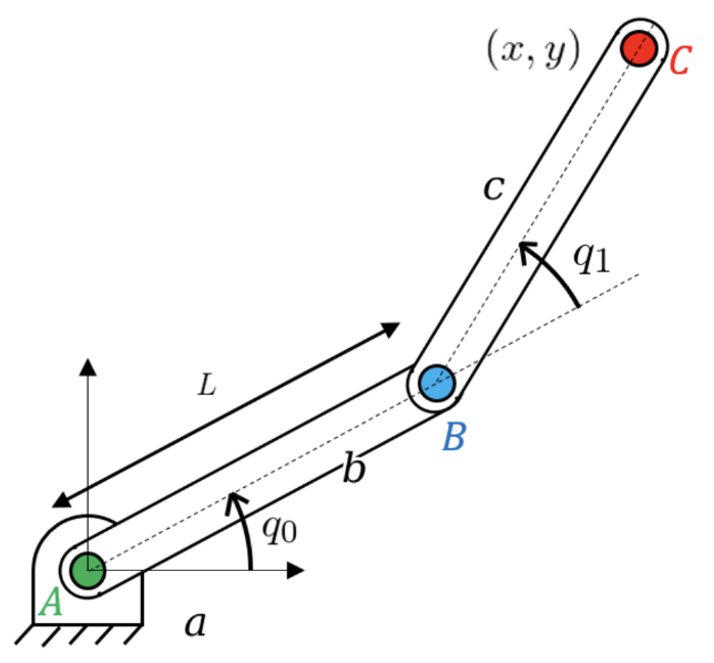
Some observations about the above:

The transforms $\{{}^aX^0, {}^bX^1, {}^cX^2\}$ are pure translations.
The transforms $\{{}^0X^b(q_0), {}^1X^c(q_1)\}$ are rotations parametrized by real numbers $(q_0, q_1)$ .
The superscripts on the RHS read out a path $a \to 0 \to b \to 1 \to c \to 2$ , which cleanly collapses to the LHS ${}^aX^2$ .

Remark. The pose of a single free body has six parameters—three for its position, and three for its orientation. But in Drake, the pose is represented using seven parameters, because the orientation is expressed using quaternions.

§ Inverse Kinematics

As one might expect, inverse kinematics can have many solutions (or none) and is very hard to compute exactly.

One could use analytic approaches to find one of the (usually many!) exact solutions to an inverse kinematics problem. But for systems with many parameters—such as our Kuka IIWA manipulator—this is not a feasible approach.

Next lecture, we'll discuss numerical approaches for estimating a solution to an inverse kinematics problem.

§ Differential Kinematics: Analytic Jacobian

Back to something easy. From forward kinematics, we know that for any body $B$ with $k$ parameters $q$ that define its pose, there is a map $f_{\mathrm{kin}}^B \colon \mathbb{R}^k \to \mathbb{R}^{3 + \ell}$ such that $X^B = f_{\mathrm{kin}}^B(q)$ . We can now differentiate this map to achieve:

\mathrm{d}X^B = \frac{\partial f_{\mathrm{kin}}^B(q)}{\partial q} \mathrm{d}q = J^B(q) \mathrm{d}q, ~ \text{ where } J^B(q) \text{ is the } \textbf{Analytic Jacobian.}

In particular, the analytic Jacobian is a derivative of a pose parametrization. Explicitly,

x(q) = \begin{bmatrix} p(q) \\ \phi(q) \end{bmatrix} \text{ where } p(q) \in \mathbb{R}^3 \text{ and } \phi(q) \in \mathbb{R}^{\ell},

where $\ell$ depends on the choice of orientation parametrization. For example, roll-pitch-yaw would require $\ell = 3$ , whereas quaternions would yield $\ell = 4$ , and rotation matrices would yield $\ell = 9$ .

It then follows that $J^B(q)$ and $\mathrm{d}q$ look like:

J^B(q) = \frac{\partial x}{\partial q} = \begin{bmatrix} \partial p/\partial q_1 & \partial p/\partial q_2 & \cdots & \partial p/\partial q_k \\ \partial \phi/\partial q_1 & \partial \phi/\partial q_2 & \cdots & \partial \phi/\partial q_k \\ \end{bmatrix} \in \mathbb{R}^{(3 + \ell) \times (k)} ~ \text{ and } ~ \mathrm{d}q = \begin{bmatrix} \mathrm{d}q_1 \\ \mathrm{d}q_2 \\ \vdots \\ \mathrm{d}q_k \end{bmatrix} \in \mathbb{R}^k.

For the simplified 2D Kuka IIWA from earlier (with $L = 1$ ), (warning: AI-generated) widget below shows how $J^C(q)$ depends on the choice of orientation parametrization.

§ Differential Kinematics: Geometric Jacobian

There's a nice simplifying trick, though. Whereas orientation has many different parametrizations—all of them flawed—velocity (as in, translational and rotational velocity combined) has a very natural $6$ -variable parametrization: the spatial velocity.

Definition. The spatial velocity of $B$ relative to $A$ is:

\frac{\mathrm{d}}{\mathrm{d}t} {}^AX^B_F = {}^AV^B_F = \begin{bmatrix} {}^A\omega^B_F \\ {}^Av^B_F \end{bmatrix} = \begin{bmatrix} {}^A\omega^B_{F, x} \\ {}^A\omega^B_{F, y} \\ {}^A\omega^B_{F, z} \\ {}^Av^B_{F, x} \\ {}^Av^B_{F, y} \\ {}^Av^B_{F, z} \end{bmatrix} \in \mathbb{R}^6,

where ${}^A\omega^B_F \in \mathbb{R}^3$ is angular velocity, and ${}^Av^B_F \in \mathbb{R}^3$ is translational velocity.

Remark. Recall that ${}^A\omega^B_F \in \mathbb{R}^3$ points along the axis of rotation with magnitude given by the angular speed. Equivalently, if

{}^A\omega^B_F = \begin{bmatrix} {}^A\omega^B_{F, x} \\ {}^A\omega^B_{F, y} \\ {}^A\omega^B_{F, z} \end{bmatrix} \in \mathbb{R}^3,

that means the rotation is equivalent to the composition of a rotation with speed ${}^A\omega^B_{F, x}$ about the $x$ -axis, a rotation with speed ${}^A\omega^B_{F, y}$ about the $y$ -axis, and a rotation with speed ${}^A\omega^B_{F, z}$ about the $z$ -axis.

Then $J^B(q)$ is not very hard to compute; the $i^{\text{th}}$ column is an $\mathbb{R}^6$ -vector that reads the rotational and translational velocities incurred by changing the $i^{\text{th}}$ parameter $q_i$ .

For example, for revolute joints (i.e., every joint $q_i$ can only rotate about a line $\hat{z}_i$ ), we have:

J^B(q) = \begin{bmatrix} \hat{z}_1 & \hat{z}_2 & \cdots & \hat{z}_k \\ \hat{z}_1 \times {}^{J_1}p^B & \hat{z}_2 \times {}^{J_2}p^B & \cdots & \hat{z}_k \times {}^{J_k}p^B \end{bmatrix} \in \mathbb{R}^{6 \times k} ~ \text{ and } ~ \mathrm{d}q = \begin{bmatrix} \mathrm{d}q_1 \\ \mathrm{d}q_2 \\ \vdots \\ \mathrm{d}q_k \end{bmatrix} \in \mathbb{R}^k.

When parametrizing velocities in this way, the $J^B(q)$ we achieve is specifically called the Geometric Jacobian.

Notice how each joint gets one column, and the height of the geometric Jacobian is always $6$ , independent of how we internally represent the end effector's orientation.

Problem. Recall the simplified 2D Kuka IIWA from earlier, specifically in the case where both rods have length $L = 1$ . What is the geometric Jacobian $J^C(q)$ of the tip $C$ ?

Solution: There are $k = 2$ joints, and they are both revolute joints. Applying the formula above, we find:

J^C(q) = \begin{bmatrix} 0 & 0 \\ 0 & 0 \\ 1 & 1 \\ -\sin(q_0) - \sin(q_0 + q_1) & -\sin(q_0 + q_1) \\ \cos(q_0) + \cos(q_0 + q_1) & \cos(q_0 + q_1) \\ 0 & 0 \end{bmatrix} \in \mathbb{R}^{6 \times 2}.

Check this for yourself; you can also play around with the (warning: AI-generated) widget below.

Note that the angular speed is not factored into $J^C(q)$ , because it's factored into $\mathrm{d}q$ instead. $\blacksquare$

You can also check for yourself that the dimensions of the geometric Jacobian of the IIWA are $6 \times 7$ .

§ Inverse Differential Kinematics: Pseudo-Inverse

Inverse differential kinematics is actually not so hard; from the relationship $\mathrm{d}X^B = J^B(q) \mathrm{d}q$ , it follows that $\mathrm{d}q = J^B(q)^{-1}\mathrm{d}X^B$ .

But this doesn't actually work as written, because $J^B(q)^{-1}$ need not exist, because the geometric Jacobian might not be square. (In general, its dimensions are $6 \times k$ , where $k$ is the number of joints.)

The fix, in general, is to take inspiration from Lecture 23 of 18.650, on linear regression.

In linear regression, we seek parameters $\beta \in \mathbb{R}^k$ such that $\mathbb{X}\beta \in \mathbb{R}^n$ is as close to $Y \in \mathbb{R}^n$ as the column space of $\mathbb{X}$ allows.
- There, $\mathbb{X}$ has full column rank, but with $n > k$ there is usually no exact solution to $\mathbb{X}\beta = Y$ .
- In this case, the desired parameter is $\beta = (\mathbb{X}^{\top}\mathbb{X})^{-1}\mathbb{X}^{\top}Y$ .
In this class, we seek an input $\mathrm{d}q$ such that $J \mathrm{d}q$ is as close to $\mathrm{d} X^B$ as the column space of $J$ allows.
- Here, $J$ usually has full row rank, meaning exact solutions $\mathrm{d}q$ to $J\mathrm{d}q = \mathrm{d}X^B$ exist (many, when $k > 6$ ).
- In this case, the desired input is the exact solution with $\|\mathrm{d}q\|$ minimized, and it looks like $\mathrm{d}q = J^{\top}(JJ^{\top})^{-1} \mathrm{d} X^B$ .

Definition. The Moore-Penrose Pseudo-Inverse $J^+$ of a matrix $J$ has two versions, depending on the rank of $J$ .

If $J$ has full column rank (as in regression), then $J^+ := (J^{\top}J)^{-1}J^{\top}$ , a left inverse ( $J^+J = I$ ).
If $J$ has full row rank (as in this class), then $J^+ := J^{\top}(JJ^{\top})^{-1}$ , a right inverse ( $JJ^+ = I$ ).

Remark. Suppose $J \colon \mathbb{R}^n \to \mathbb{R}^m$ is full row rank with $n > m$ and has null space $W$ . Then the pseudo-inverse $J^+$ must be a bijection from $\mathbb{R}^m$ to $W^{\perp} \subseteq \mathbb{R}^n$ , as shown in the image below.

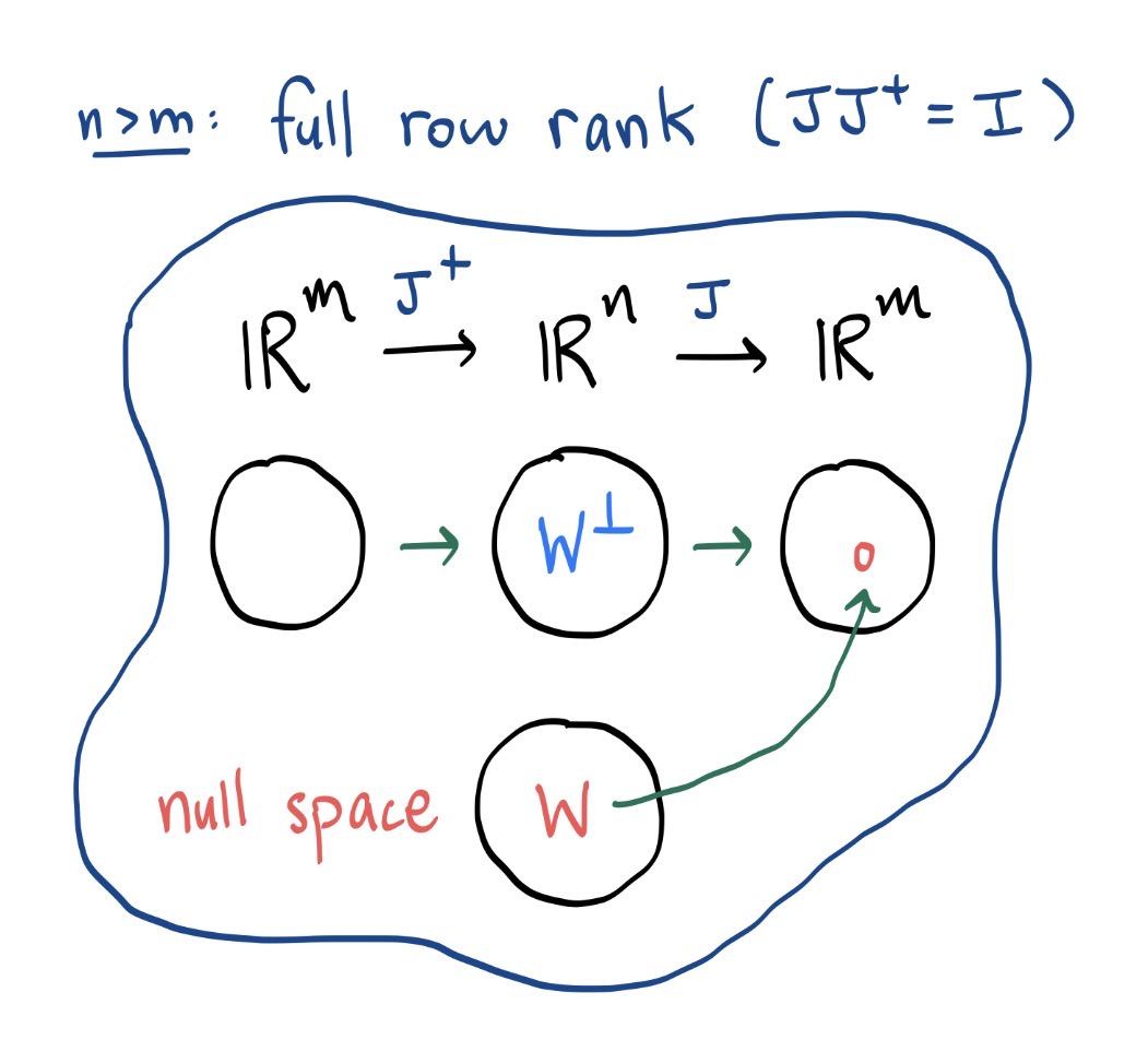
CYU: Explain why the map $M \colon \mathbb{R}^n \to \mathbb{R}^n$ given by $M := I - J^+J$ projects vectors $x \in \mathbb{R}^n$ onto the null space of $J$ .

Example. Some examples of whether $J$ has full column rank or full row rank.

For the Kuka IIWA, the geometric Jacobian is $6 \times 7$ , so it is usually full row rank, and we use $J^+ := J^{\top}(JJ^{\top})^{-1}$ .
For the simplified 2D Kuka IIWA, the geometric Jacobian is $6 \times 2$ , so it is full column rank, and we use $J^+ = (J^{\top}J)^{-1}J^{\top}$ .
- … but if we isolate only the relevant rows $v_x$ and $v_y$ , the geometric Jacobian is $2 \times 2$ , and now $J^+ = J^{-1}$ plainly.

And here's the property of $J^+$ that makes it so useful, as in both 18.650 and this class.

Theorem. (Pseudo-Inverse Approximation) For any matrix $J$ and vector $b$ (with appropriate dimensions), the vector $x^* := J^+b$ is the vector with minimum magnitude across all vectors that minimize $\|Jx - b\|$ . In particular,

If the column space of $J$ does not contain $b$ , then $x^* := J^+b$ is such that $\|Jx - b\|$ is minimized.
If the column space of $J$ contains $b$ (that is, $\|Jx - b\|$ can be zero), then $x^* := J^+b$ is the solution to $Jx = b$ minimizing $\|x\|$ .

§ Inverse Differential Kinematics: Singularities and Damping

But there's still an issue with the pseudo-inverse as stated above; its values can explode near singularities.

Definition. We say there is a singularity when the rows of $J^B(q)$ for the velocities we want to control are not full row rank.

Example. In the two-rod example from earlier, when considering only the gripper's $(x, y)$ velocity, one singularity occurs when $q_1 = 0$ : both joints can then only move the gripper perpendicular to the arm.

Observe this in the (warning: AI-generated) widget below. When $q_1$ approaches $0$ , and the desired $\mathrm{d}X$ points outside the shaded ellipse, the computed $(\mathrm{d}q_0, \mathrm{d}q_1)$ values blow up.

The fix for this problem is also inspired by 18.650; it's equivalent to adding a ridge regression term.

Definition. The damped pseudo-inverse of $J$ (for any $J$ , given $\lambda > 0$ ) is:

J^* = J^{\top}(JJ^{\top} + \lambda I)^{-1}.

The $\lambda I$ term prevents things from exploding when $JJ^{\top}$ is close to zero in some directions. You can also observe this using the widget above; the $\lambda I$ sacrifices output accuracy in favor of controlled $(\mathrm{d}q_0, \mathrm{d}q_1)$ values.

Remark. The existence of a singularity is not enough to cause concern if that singularity occurs momentarily.

For example, if $q_1$ gradually decreases from $+10^{\circ}$ to $-10^{\circ}$ , then there is a moment when $q_1 = 0^{\circ}$ and a singularity occurs. But such a moment is instantaneous; the pre-existing momentum of the robot allows it to pass the singularity unharmed.

§ Addendum: Velocities and Change-Of-Frame

The lecture also covers the following information about how velocities change between frames.

Theorem. (Monogram Velocities) The following identities are all true.

(Change of Frame) We have ${}^Av^B_G = {}^GR^F {}^Av^B_F$ and ${}^A\omega^B_G = {}^GR^F {}^A\omega^B_F$ .
(Additivity) We have ${}^A\omega^B_F + {}^B\omega^C_F = {}^A\omega^C_F$ and ${}^Av^C_F = {}^Av^B_F + {}^Bv^C_F + {}^A\omega^B_F \times {}^Bp^C_F$ .
(Inverse) We have ${}^A\omega^B_F = -{}^B\omega^A_F$ and ${}^Av^B_F = -{}^Bv^A_F - {}^A\omega^B_F \times {}^Bp^A_F$ .

Proof: The simplified 2D Kuka IIWA example from earlier is a prototype to use when thinking through these identities.

For the identity ${}^Av^C_F = {}^Av^B_F + {}^Bv^C_F + {}^A\omega^B_F \times {}^Bp^C_F$ , for example, recall that ${}^Bv^C_F$ only captures the movement of tip $C$ in the frame of joint $B$ . So if only joint $B$ is rotating, then ${}^Bv^C_F$ is zero, even though $C$ is moving in the frame of $A$ .

To account for the movement of tip $C$ caused by the rotation of frame $B$ , we must add the term ${}^A\omega^B_F \times {}^Bp^C_F$ . (You can check that the proportionalities make sense.) $\blacksquare$