MIT 18.701 — Lecture 19

Applications of the Spectral Theorem

Today will be dedicated to applying the Spectral Theorem in three broader contexts.

§ Spectral Application #1: Classifying Quadric Surfaces

We've done enough foreshadowing already.

In Section 16.3, we foreshadowed how all quadratic polynomials $\mathbb{R}^n \to \mathbb{R}$ look like:
$\text{quadratic polynomials} = \underbrace{\left(\sum_{i, j} A_{i, j} x_i x_j\right)}_{\text{degree 2 terms}} + \underbrace{\left(\sum_{i} b_i x_i \right)}_{\text{degree 1 terms}} \ + \ \left(c\right) = x^{\top}Ax + b^{\top}x + c.$
In Section 17.5, we foreshadowed how the signature of $A$ encodes its behavior.

Let's get to the punchline of this foreshadowing.

Definition (Quadric Surface). A quadric surface in $\mathbb{R}^n$ is a subset of the form $\{x \in \mathbb{R}^n \mid x^{\top}Ax + b^{\top}x + c = 0 \}$ for some symmetric matrix $A \in \mathbb{R}^{n \times n}$ , $b \in \mathbb{R}^n$ , and $c \in \mathbb{R}$ .

Example. We already know the $n = 1$ and $n = 2$ cases from high school.

In $n = 1$ , quadric surfaces are either pairs of points, single points, the empty set, or all of $\mathbb{R}$ .
In $n = 2$ , quadric surfaces are conics: ellipses, hyperbolas, and the degeneracies.

We now use a special case of the Spectral Theorem in the context of $\mathbb{R}$ .

Theorem. (Spectral Theorem over $\mathbb{R}^n$ ) If $A \in \mathbb{R}^{n \times n}$ is symmetric, its eigenvectors form an orthonormal basis.

In other words, there exists some $T \in O_n(\mathbb{R})$ such that $T^{\top}AT = \Lambda$ , where $\Lambda$ is diagonal. Thus,

\begin{align*}& x^{\top}Ax + b^{\top}x + c = 0 \\ \iff ~~ & \textcolor{#bf0140}{(T^{-1}x)}^{\top} (T^{\top}AT)\textcolor{#bf0140}{(T^{-1}x)} + (T^{\top}b)^{\top}\textcolor{#bf0140}{(T^{-1}x)} + c = 0 & \text{ by plain computation } \\ \iff ~~ & y^{\top}\Lambda y + (T^{\top}b)^{\top}y + c = 0 & \text{ where } \textcolor{#bf0140}{y = T^{-1}x} \\ \iff ~~ & \left(\lambda_1y_1^2 + \dots + \lambda_ny_n^2\right) + \left(b_1'y_1 + \dots + b_n'y_n\right) + c = 0\end{align*}

The point is that $y = T^{-1}x$ represents an orthonormal change of basis because $T \in O_n(\mathbb{R})$ . Therefore,

Theorem. (Quadric Classification) All quadric surfaces, up to an orthonormal change of basis, look like:

\left\{ y \in \mathbb{R}^n : \left(\sum_{i = 1}^n \lambda_i y_i^2\right) + \left(\sum_{i = 1}^n b_i y_i \right) + c = 0 \right \}

Furthermore, if $\det A \neq 0$ , then each $\lambda_i$ is nonzero, so we can complete the square, leaving $\sum_{i = 1}^n \lambda_i y_i^2 = k$ for some constant $k$ . When $k \neq 0$ , we can also scale, yielding…

Theorem. (Non-Singular Quadric Classification) All nonsingular quadric surfaces—those with $\det A \neq 0$ and $k \neq 0$ —are affinely equivalent to:

\left\{ y \in \mathbb{R}^n : \sum_{i = 1}^n \lambda_i y_i^2 = 1 \right \}, \text{ where each $\lambda_i$ is either $+1$ or $-1$.}

Some corollaries of these observations:

There are only $n + 1$ non-singular quadric surfaces in $\mathbb{R}^n$ .
Parabolas are a degeneracy! They correspond to a singular choice of $A$ .
Almost all randomly chosen $\mathbb{R}^3$ quadric surfaces (say, $67xy + 41z^2 - 14yz + 34x = 1$ , for example) are affinely equivalent to one of the following: $x^2 + y^2 + z^2 = 1 ~~ \text{ or } ~~ x^2 + y^2 - z^2 = 1 ~~ \text{ or } ~~ x^2 - y^2 - z^2 = 1$ .

§ Spectral Application #2: Principal Component Analysis

For this section, here's the setup:

Setup. Take $n$ random variables $\{X_i\}_{i = 1}^n$ in a column vector $X \in \mathbb{R}^n$ .
Normalize the $X_i$ so that $\mathbb{E}[X_i] = 0$ for all $i$ . (In other words, $\mathbb{E}[X] = 0$ .)

We'll first build all necessary mathematical foundations, up to the Rayleigh-Ritz theorem.

Definition (Variance, Covariance, Covariance Matrix). Let $A$ and $B$ be random variables in $X$ .

The variance of $A$ is $\Var(A) := \mathbb{E}[A^2] - \mathbb{E}[A]^2$ .
When $A$ is normalized so that $\mathbb{E}[A] = 0$ , we have $\Var(A) = \mathbb{E}[A^2]$ .
The covariance of $A$ and $B$ is $\mathrm{Cov}(A, B) := \mathbb{E}[AB] - \mathbb{E}[A]\mathbb{E}[B]$ .
When $A$ and $B$ are normalized so that $\mathbb{E}[A] = \mathbb{E}[B] = 0$ , we have $\mathrm{Cov}(A, B) = \mathbb{E}[AB]$ .
The covariance matrix of $X$ is $\mathrm{Cov}(X) := (\mathrm{Cov}(X_i, X_j))_{i, j}$ .
When $X$ is normalized so that $\mathbb{E}[X] = 0$ , we have $\mathrm{Cov}(X) = \mathbb{E}[XX^{\top}]$ .

Theorem. (Variance of Linear Combinations) Let $M := \mathrm{Cov}(X)$ . Then for any $c \in \mathbb{R}^n$ , we have $\Var(c^{\top}X) = c^{\top}Mc$ .

Proof: Just plain computation.

\Var(c^{\top}X) = \Var\left(\sum_{i = 1}^n c_iX_i\right) = \mathbb{E}\left [ \left(\sum_{i = 1}^n c_i X_i \right)^2 \right ] = c^{\top}Mc. ~~~ \blacksquare

Theorem. (Rayleigh-Ritz) Let $M$ be any symmetric matrix with normalized eigenvectors $\{v_1, \dots, v_n\}$ and corresponding eigenvalues $\lambda_1 \geq \dots \geq \lambda_n$ . Then:

\max_{c \in \mathbb{R}^n \setminus \{0\}} \dfrac{c^{\top}Mc}{c^{\top}c} = \lambda_1, ~ \text{ and more generally, } ~ \max_{\substack{c \in \mathbb{R}^n \setminus \{0\} \\ c \perp v_i \text{ for all } i < k}} \dfrac{c^{\top}Mc}{c^{\top}c} = \lambda_k.

Proof: By the Spectral theorem, $\{v_1, \dots, v_n\}$ is an orthonormal basis. Writing $c = \sum_{i = 1}^n \alpha_i v_i$ yields:

\dfrac{c^{\top}Mc}{c^{\top}c} = \dfrac{\sum_{i = 1}^n \alpha_i^2 \lambda_i}{\sum_{i = 1}^n \alpha_i^2} = \sum_{i = 1}^n \left(\dfrac{\alpha_i^2}{\sum_{j = 1}^n \alpha_j^2}\right) \lambda_i.

This is a weighted average of $\{\lambda_i\}_{i = 1}^n$ , and the maximum possible weighted average is $\max\{\lambda_i\}_{ i = 1}^n = \lambda_1$ .

More generally, when $c \perp v_i$ for all $i < k$ , we're forced to have $\alpha_i = 0$ for all $i < k$ . Then we instead have a weighted average of $\{\lambda_i\}_{i = k}^n$ , for which the maximum possible value is $\lambda_k$ . $\blacksquare$

Mathematics aside, here's what we wish to do with our random variables $\{X_i\}_{i = 1}^n$ from earlier.

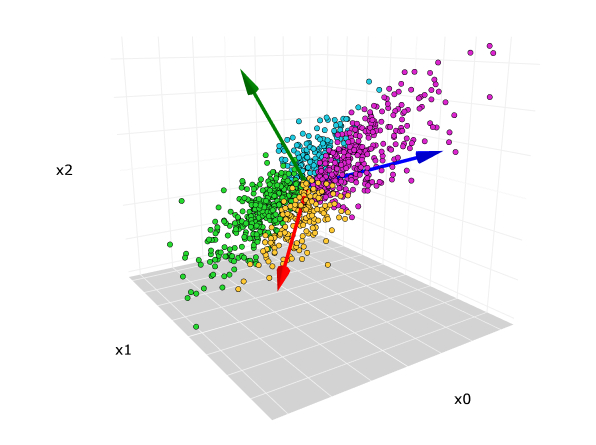
Intuition. Many samples from $X$ form a point cloud in $\mathbb{R}^n$ . We wish to look at
this point cloud from a certain angle—a certain orthonormal basis, perhaps—so that
the axes of our orthonormal basis point in “meaningful directions”.

What qualifies as a “meaningful direction”, then? The Rayleigh-Ritz theorem proposes a good candidate.

Theorem. (Rayleigh-Ritz Corollary) Let $M$ be the covariance matrix of $X$ . Then $\frac{\Var(c^{\top}X)}{c^{\top}c}$ is maximized when $c$ is the eigenvector of $M$ with greatest eigenvalue.

Think of our point cloud as a messy ellipsoid centered at the origin. Then the $c$ that maximizes $\frac{\Var(c^{\top}X)}{c^{\top} c}$ will be the $c$ that points along the highest-variance axis of $X$ —that is, the longest axis of the ellipsoid!

In fact, the more general case of Rayleigh-Ritz indicates that the set of all eigenvectors of $M$ will point along orthogonal axes of this ellipsoid! In conclusion,

— Conclusion (PCA) —

Given a point cloud $X$ of data with covariance matrix $M$ ,
we can identify the most “principal components” of the point cloud
by picking out the eigenvectors of $M$ with the greatest eigenvalues.

Naturally, the strategy of using the eigenvectors of $M$ to analyze $X$ is called Principal Component Analysis (PCA).

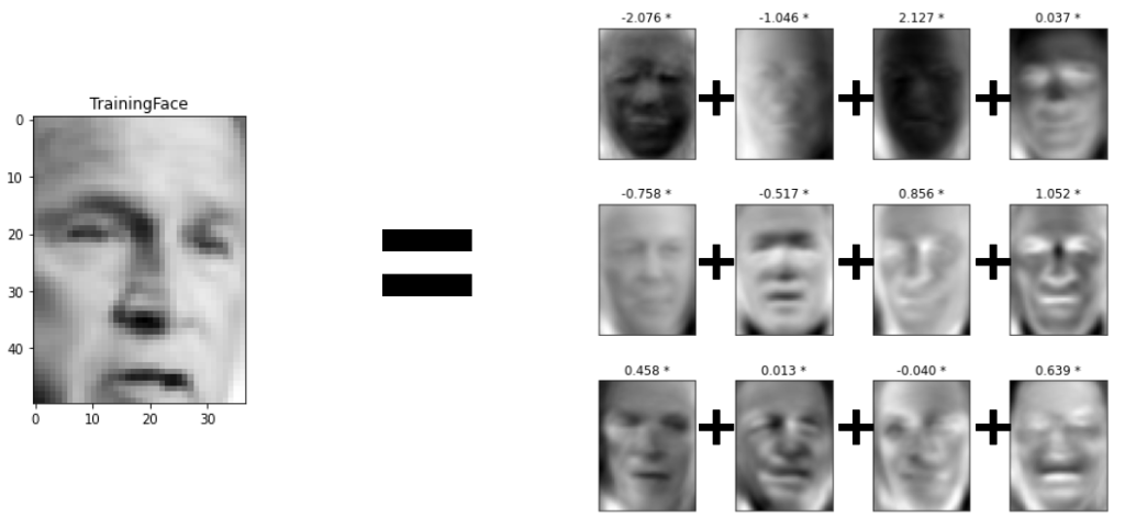
In the particular context of facial recognition, eigenfaces are a set of eigenvectors whose linear combination with unique coefficients yields distinct faces.

§ Spectral Application #3: Singular Value Decomposition

Here's the setup this time.

Setup. We have $n$ normalized random variables $\{X_i\}_{i = 1}^n$ , and we sample each one $m$ times.
This gives us a matrix $X \in \mathbb{R}^{m \times n}$ , where $X_{i, j}$ gives the $i^{\text{th}}$ sample of $X_j$ .

We'll first state the necessary mathematics, then show its applications, and finally prove the mathematics.

Definition (Sample Covariance). The sample covariance matrix of $X$ is the $n \times n$ matrix $\mathrm{Cov}(X) := \frac{1}{m - 1} X^{\top}X$ .

Intuitively, $\mathrm{Cov}(X)_{i, j}$ gives the sample covariance of $X_i$ and $X_j$ .

Theorem. (Singular Value Decomposition) Every matrix $A \in \mathbb{R}^{m \times n}$ factors in the following way:

A = V \Sigma W^{\top} ~~ \text{ for some } ~~ V \in O_m(\mathbb{R}), ~ W \in O_n(\mathbb{R}), \text{ and diagonal } \Sigma \in \mathbb{R}^{m \times n}.

If $\Sigma$ has diagonal entries $\sigma_1 \geq \sigma_2 \geq \dots \geq 0$ , then we say $\{\sigma_i\}$ are the singular values of $A$ .

If $X$ factors in this way as $X = V \Sigma W^{\top}$ with singular values $\{\sigma_i\}$ , then the sample covariance matrix is:

\mathrm{Cov}(X) = \dfrac{1}{m - 1} (W \Sigma^{\top} V^{\top}) (V \Sigma W^{\top}) = \dfrac{1}{m - 1} W (\Sigma^{\top} \Sigma)W^{\top} = \dfrac{1}{m - 1} W \left[\begin{smallmatrix} \sigma_1^2 & \cdots & 0 \\ \vdots & \ddots & \vdots \\ 0 & \cdots & \sigma_n^2 \end{smallmatrix}\right]W^{\top}

The way $\Sigma^{\top}\Sigma$ is written above assumes $m \geq n$ . If $m < n$ , then the remaining $n - m$ diagonal entries are zeroes.

— Conclusion (SVD on Covariance Matrices) —

Consider a matrix $X \in \mathbb{R}^{m \times n}$ of data. Assume $m \geq n$ .
Factor $X$ as $V \Sigma W^{\top}$ with singular values $\sigma_1 \geq \sigma_2 \geq \dots \geq 0$ .

Then $\mathrm{Cov}(X)$ has eigenvalues $\left\{\tfrac{\sigma_i^2}{m - 1}\right\}_{i = 1}^n$ and eigenvectors being the columns of $W$ .

(If $m < n$ , then the remaining $n - m$ eigenvalues are zeroes.)

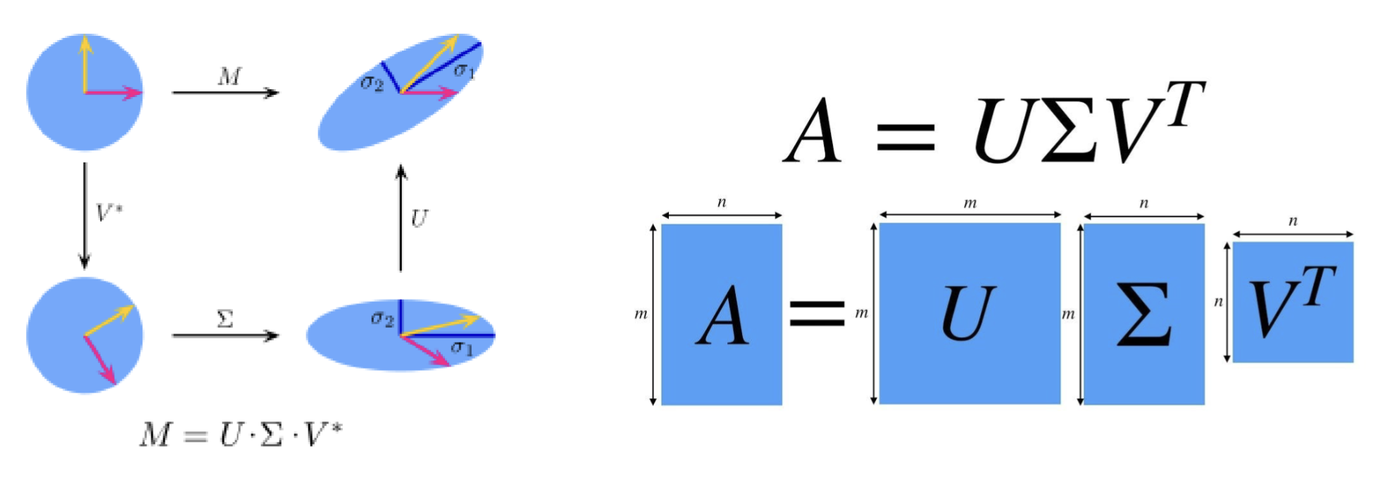
Some useful diagrams depicting object-level examples of what SVD does.

Some good things to keep in mind while we prove SVD.

For orthogonal matrices $V$ and $W$ , we always have $V^{\top} = V^{-1}$ and $W^{\top} = W^{-1}$ .
Recall $A \in \mathbb{R}^{m \times n}$ is a map $A: \mathbb{R}^n \to \mathbb{R}^m$ , so $W$ and $V$ are operators on the domain and codomain, respectively.

Proof: Assume without loss of generality that $n \leq m$ . (If instead $n \geq m$ , work with $A^{\top}$ instead of $A$ .)

We begin by rephrasing our win condition.

Claim. It suffices to find orthonormal bases $\{v_1, \dots, v_m\} \subseteq \mathbb{R}^m$ and $\{w_1, \dots, w_n\} \subseteq \mathbb{R}^n$ and constants $\{\sigma_1, \dots, \sigma_n\}$ such that $Aw_i = \sigma_i v_i$ for all $i = 1, 2, \dots, n$ .

Proof: Use the $\{v_i\}_{i = 1}^m$ and $\{w_i\}_{i = 1}^n$ as columns of $V$ and $W$ , and use the $\{\sigma_i\}_{i = 1}^n$ as the diagonal of $\Sigma$ .

To show $A = V\Sigma W^{\top}$ , it suffices to check that $A$ and $V \Sigma W^{\top}$ agree on the images of every element in some basis of the domain $\mathbb{R}^n$ . Let's use the basis $\{w_i\}_{i = 1}^n$ .
$(1) ~~~ A(w_i) = \sigma_i v_i \text{ by assumption.} ~~~~~~~~~~~ (2) ~~~ V \Sigma W^{\top}(w_i) = \sigma_i v_i \text{ by computation.}$
Hooray—they match. $\square$

Observe the following properties of $A^{\top}A \in \mathbb{R}^{n \times n}$ .

Since $A^{\top}A$ is symmetric, the Spectral theorem says its eigenvectors form an orthonormal basis.
Thus, we may take $\{w_i\}_{i = 1}^n$ to be this orthonormal basis. (This move is forced—why?)
Since $A^{\top}A$ is positive semidefinite, the eigenvalues $\{\lambda_i\}_{i = 1}^n$ of $A^{\top}A$ are nonnegative.
Thus, we may take $\{\sigma_i\}_{i = 1}^n$ to be $\sigma_i = \sqrt{\lambda_i}$ for all $i$ . (This move is forced—why?)

Great! We've already found $\{w_i\}_{i = 1}^n$ and $\{\sigma_i\}_{i = 1}^n$ .

For $\{v_i\}_{i = 1}^m$ , we'll just take $v_i = \frac{Aw_i}{\sigma_i}$ for $i \leq n$ , then fill in the rest arbitrarily (maintaining orthonormality).

Well, it's pretty obvious that $Aw_i = \sigma_i v_i$ will hold for all $i$ . Now we just need to show $\{v_i\}_{i = 1}^m$ is orthonormal.

\langle v_i, v_j \rangle = v_i^{\top}v_j = \frac{w_j^{\top}A^{\top}Aw_i}{\sigma_i \sigma_j} = \frac{w_j^{\top}(\sigma_i^2 w_i)}{\sigma_i \sigma_j} = \frac{\sigma_i}{\sigma_j}\langle w_j, w_i \rangle = \begin{cases} 1 & \text{ if } i = j \\ 0 & \text{ if } i \neq j \end{cases}

We've checked everything we needed, so we're done. $\clubsuit$

Well, okay, fine—there's one issue we missed, shown in orange. If $\sigma_i = 0$ , then $v_i = \frac{Aw_i}{\sigma_i}$ doesn't make sense. Fortunately, if $\sigma_i = 0$ , there's an easy fix.

\sigma_i = 0 . ~ \implies ~ A^{\top}Aw_i = 0. ~ \implies ~ \langle w_i, A^{\top}Aw_i \rangle = 0. ~ \implies ~ \langle Aw_i, Aw_i \rangle = 0. ~ \implies ~ Aw_i = 0.

Thus, the constraint $Aw_i = \sigma_i v_i$ holds trivially—again just pick $v_i$ arbitrarily, maintaining orthonormality. $\blacksquare$

Unlike some of our previous “factorization” theorems, this one applies to all matrices!

Remark. Despite how long the above proof is, it's actually extremely motivated—in particular, $AA^{\top}$ and $A^{\top}A$ tell us what $V$ , $W$ , and $\Sigma$ have to be, and then it remains to check that everything remains consistent.

Hint: It is rumored that the SVD may be useful for Problem Set #10.

§ Linear Groups

We're about to transition to a new topic: embedding groups into geometric objects.

Example. There exists a natural bijection $SO_2(\mathbb{R}) \leftrightarrow S^1$ , where $S^1$ is the unit circle.

The interesting point, however, is that it's surprisingly difficult to embed $SO_3(\mathbb{R})$ into a geometric object!

Here are some failed attempts:

Every rotation in $SO_3(\mathbb{R})$ can be described by an axis $v \in S^2$ and an angle $\theta \in S^1$ . Thus, $SO_3(\mathbb{R}) \cong S^2 \times S^1$ .
- Unfortunately, this “bijection” has a lot of messy non-injectivity! For example, $v$ and $-v$ represent the same axis.
Every rotation in $SO_3(\mathbb{R})$ can be described using roll, pitch, and yaw. Thus, $SO_3(\mathbb{R}) \cong S^1 \times S^1 \times S^1$ .
- When built in real life, this parametrization can cause gimbal lock to occur!
- Famously, gimbal lock caused problems on the Apollo 11 Moon mission.

Spoilers: it turns out $S^3$ and the quaternions will be the most natural parametrization of $SO_3(\mathbb{R})$ .