MIT 6.790 — Lecture 12

Neural Networks

§ Neurons

Recall from Lecture 11 that the hypothesis class specified by regression models does not contain a hypothesis that can correctly model two-variable XOR; the data pictured below is not linearly separable.

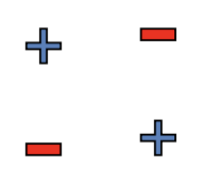
We need more general models than regression models. In come neural networks.

Definition. A single neuron is a function $h \colon \mathbb{R}^d \to \mathbb{R}$ , made up of two parts:

The pre-activation of a neuron is $a(x) := w_0 + w^{\top} x$ ; that is, a weighted sum of $d$ inputs plus a bias $w_0$ .
The activation / output of a neuron is $h(x) := g(a(x))$ , where $g \colon \mathbb{R} \to \mathbb{R}$ is an activation function.

Some common choices of activation functions include:

\text{(sigmoid $\sigma$)} ~~~ g(t) := \frac{1}{1 + e^{-t}} ~~~ \parallel ~~~ g(t) := \tanh(t) = \frac{e^t - e^{-t}}{e^t + e^{-t}} ~~~ \parallel ~~~ g(t) := \mathrm{sgn}(t) ~~~ \parallel ~~~ \text{(ReLU)} ~~~ g(t) := \max(0, t)

Remark. Note that $\tanh(x) = 2 \sigma(2x) - 1$ , so the sigmoid and tanh activations are roughly the same.

§ Neural Networks: XOR Example

Note that a single neuron with sigmoid activation is identical to logistic regression. This means that a single neuron isn't enough to model two-variable XOR. One fix, however, is to use a linear classifier over a hardcoded feature space.

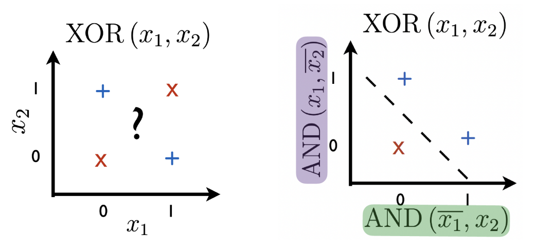
As shown above, the following $\mathbb{R}^2 \to \mathbb{R}^2$ feature map allows us to compute $\mathrm{XOR}(x_1, x_2)$ via a linear classifier.

\Phi \colon (x_1, x_2) \mapsto \left(\mathrm{AND}(x_1, \overline{x}_2), \mathrm{AND}(\overline{x}_1, x_2)\right).

In the diagram below, we represent the process of first converting our inputs $(x_1, x_2)$ into features $\left(\mathrm{AND}(x_1, \overline{x}_2), \mathrm{AND}(\overline{x}_1, x_2)\right)$ , then using the features as inputs to the output neuron.

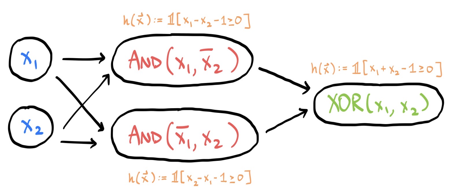
Each input $(x_1, x_2)$ is a node, each feature $\left(\mathrm{AND}(x_1, \overline{x}_2), \mathrm{AND}(\overline{x}_1, x_2)\right)$ is a node, and the output $\mathrm{XOR}(x_1, x_2)$ is a node. Furthermore, an edge $u \to v$ is drawn if $u$ is an input to the neuron whose output is $v$ .

Here's the important point: not only is the final output $\mathrm{XOR}(x_1, x_2)$ a neuron, but the intermediate feature nodes $\mathrm{AND}(x_1, \overline{x}_2)$ and $\mathrm{AND}(\overline{x}_1, x_2)$ are neurons too! Note that their activation function is $g(z) := \mathds{1}[z \geq 0]$ .

The diagram above is an example of a neural network. Let's generalize this to a definition.

§ Neural Networks: Definition

Definition. A neural network consists of one input layer, some number $L$ of hidden layers, and one output layer.

The input layer just reads in the input vector $x \in \mathbb{R}^d$ . It's the identity map $h^{(0)} \colon \mathcal{X} \to \mathbb{R}^d$ given by $h^{(0)}(x) := x$ .
The $k^{\text{th}}$ hidden layer is the map $h^{(k)} \colon \mathcal{X} \to \mathbb{R}^{N_k}$ , whose output is a neuron activation of the output of the $(k - 1)^{\text{th}}$ layer.
$h^{(k)}(x) = g\left(b^{(k)} + W^{(k)} h^{(k - 1)}(x)\right).$
Note that $N_k$ denotes the dimension of the output of $h^{(k)}$ . Equivalently, $N_k$ is the number of neurons in the $k^{\text{th}}$ layer.

By consequence, note that we must have $W^{(k)} \in \mathbb{R}^{N_k \times N_{k - 1}}$ .
The output layer is the map $h^{(L + 1)} \colon \mathcal{X} \to \mathbb{R}^{N_{L + 1}}$ . It operates just like every hidden layer; its output is the final answer.

That's a whole bunch of jargon to explain the relatively simple idea of chaining $L$ layers of neurons together.

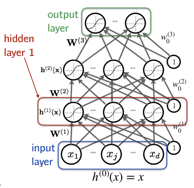
Here's how this looks in the example of the XOR neural network. Every single parameter in the neural network—that is, every value of $b^{(k)}$ and every entry of a matrix $W^{(k)}$ —is written in purple text.

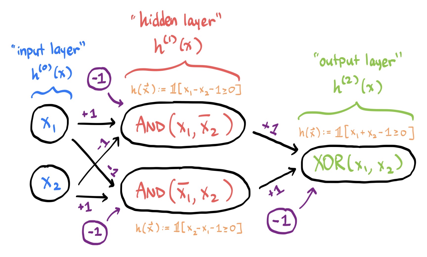
The upshot of neural networks comes from their hidden layers. Previously, we would just have to have known, somehow, that $\Phi(x) := \left(\mathrm{AND}(x_1, \overline{x}_2), \mathrm{AND}(\overline{x}_1, x_2)\right)$ would be a good set of features for encoding $\mathrm{XOR}(x_1, x_2)$ .

With neural networks, however, instead of hardcoding the best features $\Phi(x)$ (or, in the neural network analogy, the best $h^{(L)}(x)$ ) to use, we can instead learn the best features by optimizing the parameters $\{b^{(k)}, W^{(k)}\}_{k = 1}^{L + 1}$ .

Hidden layers encode features. That raises the question: are hidden layers capable of encoding any feature?

§ Neural Network Universal Approximation

The answer is yes, mostly.

Theorem. (Universal Approximation) For every continuous $f \colon [0, 1]^d \to \mathbb{R}$ and $\epsilon > 0$ , there is a function $\hat{f}$ that is a linear combination of ReLUs such that $\int_{[0, 1]^d} |f(x) - \hat{f}(x)| \, \mathrm{d}x < \epsilon$ .

Furthermore, we can upper-bound the complexity of such a function $\hat{f}$ , somewhat.

Theorem. (Universal Approximation Bound) Suppose $f \colon [0, 1]^d \to \mathbb{R}$ is 1-Lipschitz continuous—that is, $|f(x) - f(y)| \leq \|x - y\|$ for all $x, y \in [0, 1]^d$ . Then for all $\epsilon > 0$ , there is a function $\hat{f}$ that is a linear combination of order $(1/\epsilon)^d$ ReLUs such that $\int_{[0, 1]^d} |f(x) - \hat{f}(x)| \, \mathrm{d}x < \epsilon$ .

Interestingly, both of these theorems state that only one hidden layer is technically necessary—each ReLU is a single node in that layer, and the output layer is the linear combination of those nodes.

Still, though, as we'll see in future lectures, it is often useful to use more than one hidden layer, both from a computation perspective and a representation perspective.