MIT 6.790 — Lecture 8

§ Classification

Over the past few lectures on linear regression, we've assumed that the output space $\mathcal{Y}$ is $\mathbb{R}$. In classification problems, we instead take $\mathcal{Y}$ to be discrete; for now, let's further assume $\mathcal{Y}$ is binary, meaning $\mathcal{Y} = \{+1, -1\}$.

This is the setup for logistic regression, covered in Lecture 25 of 18.650. These notes will assume knowledge of that lecture.

§ Bayes Classifier

Here's the most common choice of loss function for (binary) classification problems.

Definition. The zero-one loss is $\mathcal{L}(\hat{y}, y) := \mathds{1}[\hat{y} \neq y]$. The loss equals zero if the classification was right, and one otherwise.

In this case, it's clear that the best classifier is the Bayes classifier.

Of course, the challenge is that we don't know what the distribution $[Y \mid X = x]$ exactly looks like.

§ Nearest Neighbor Classifier

Here's a simple design of a binary classifier.

Definition. Given an input space $\mathcal{X}$, impose some distance metric $d \colon \mathcal{X} \times \mathcal{X} \to \mathbb{R}^{\geq 0}$. Then predict the label $h(x)$ like so:

Identify the set $N_k(x)$ of the indices of the $k$ training points closest to $x$. Then return $h(x) = \mathrm{sgn}\left(\sum_{i \in N_k(x)} y^{(i)}\right)$.

This is called the nearest neighbor classifier (or NN, or KNN). It's simple, but slow: making a single prediction requires scanning the entire training set.

§ ERM: Linear Classifier

Let's try an ERM approach instead; here's the set of hypotheses we'll restrict ourselves to.

Definition. A linear classifier is a map $h \colon \mathcal{X} \to \{+1, -1\}$ via $h(x) := \mathrm{sgn}\left(w^{\top}x\right)$, for some parameter $w$.

Then ERM tells us we should choose $w$ to minimize the empirical risk $\widehat{\mathrm{risk}}(h_w)$, given below:

Note that $\mathcal{L}(z)$ is just a one-variable form of zero-one loss. Unfortunately, the empirical risk described above is hard to optimize (via gradient descent, say) because $\mathcal{L}(z)$ is not convex or differentiable. Here's a better alternative:

Definition. A convex variant of zero-one loss is logistic loss, given by $\mathcal{L}_{\mathrm{logistic}}(z) := \log_2(1 + e^{-z})$.

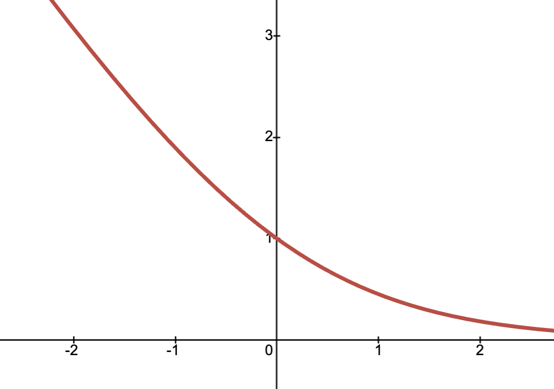
§ Addendum: Convexity

We provide a brief reminder of convexity here; it's important to know for optimization purposes.

Definition. A twice-differentiable function $f \colon \mathbb{R}^n \to \mathbb{R}$ is convex if any of the following (equivalent) statements is true.

1. We have $\nabla^2 f(x) \succeq 0$ for all $x$; that is, $\nabla^2 f(x)$ is positive semidefinite.

   • Note that $\nabla^2 f(x)$ here is the Hessian, which is the $n \times n$ matrix given by $\left[\nabla^2 f(x)\right]_{i, j} := \frac{\partial^2 f}{\partial x_i \partial x_j}(x)$.

2. We have $f\left(\lambda \cdot u + (1 - \lambda) \cdot v\right) \leq \lambda \cdot f(u) + (1 - \lambda) \cdot f(v)$ for all $u, v \in \mathbb{R}^n$ and $\lambda \in [0, 1]$.

   • That is, any line segment connecting two points on the graph of $f$ lies above the graph.

3. We have $f(u) \geq f(v) + \nabla f(v)^{\top}(u - v)$ for all $u, v \in \mathbb{R}^n$.

   • That is, the tangent plane to $f$ at $v$ lives underneath the graph of $f$ everywhere.

Here's why we care about convexity so much:

So techniques that seek out local minima (e.g., gradient descent) are really seeking out the global minimum. You can check that logistic loss is convex.

§ MLE: Logistic Regression

As in Lecture 25, we'll switch our hypothesis to be a map $p_w \colon \mathcal{X} \to [0, 1]$, where the goal is to have $p_w(x)$ be a solid approximation of $\mathbb{P}(Y = +1 \mid X = x)$. Then our classification model is $h_w(x) := \mathrm{sgn}\left(p_w(x) - \frac{1}{2}\right)$, naturally.

Specifically, we'll assume that $p_w$ takes the form $p_w(x) = \sigma\left(w^{\top}x\right)$, where $\sigma(z) := \frac{e^z}{1 + e^z}$ is the sigmoid function.

The proof is just plain computation, so we omit it. Note that this differs slightly from the result in Lecture 25 of 18.650 because of the convention that $y^{(i)} \in \{+1, -1\}$ instead of $y^{(i)} \in \{0, 1\}$.

The interesting part is the coincidence that logistic loss shows up once again. The following are therefore identical:

• Maximizing the likelihood, given a model $p_w(x) = \sigma(w^{\top}x)$ designed to approximate $\mathbb{P}(Y = +1 \mid X = x)$.

• Minimizing the logistic loss, given a hypothesis $h(x) := \mathrm{sgn}(w^{\top}x)$ designed to predict the classification of $x$.

§ Addendum: Log-Odds and Linear-Logistic Equivalence

Definition. The log-odds is defined as the value $f(x) := \log \left[ \frac{\mathbb{P}(Y = +1 \mid X = x)}{\mathbb{P}(Y = -1 \mid X = x)} \right]$.

So all of the discussion about features and kernels concerning linear regression applies equally well to logistic regression.