MIT 6.790 — Lecture 15

Double Descent and Implicit Regularization

§ Double Descent

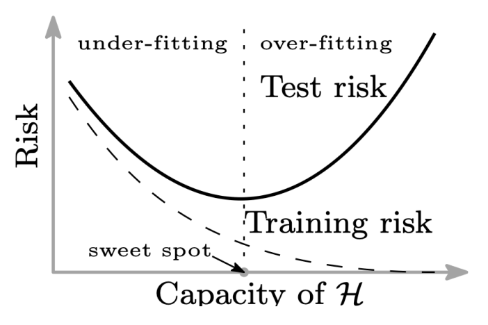
The intuition that classical statistics gives us is that models with larger hypothesis classes $\mathcal{H}$ are more prone to overfitting. In this sense, achieving zero training error via increasing the parameter count may have negative consequences on the test error.

The modern deep learning perspective, however, is that setting the parameter count even higher can contribute positively toward decreasing the test error in the long term! This phenomenon is known as double descent.

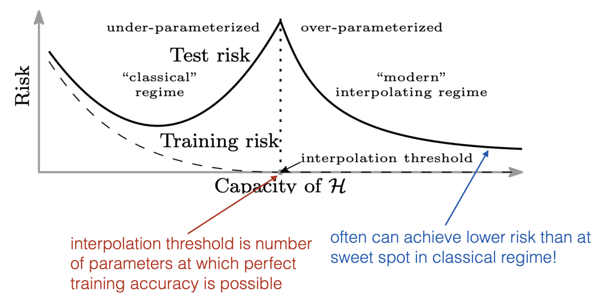
The graphs below provide some intuition for why double descent takes place.

Here's what these graphs indicate:

In the leftmost graph, the number of parameters is low, so both the training and test error are large.
In the middle graph, the number of parameters is just large enough for ERM to find a perfect interpolation through the training data—the interpolation threshold. Thus, training error is zero, but test error is large due to overfitting.
In the rightmost graph, the number of parameters is large enough for ERM to find multiple interpolations through the training data. If we add a ridge penalty $\lambda \|\theta \|^2$ to our loss function, then ERM finds the interpolation with the smallest weights, which overfits the least! So the training error is zero, and the test error is small.

Remark. Besides plain intuition, one solid argument as to why adding a ridge penalty should improve test error is the error bound we derived in Lecture 10 (restated below).

Assuming $\mathcal{L}(x, y) \in [0, 1]$ , for all $\delta \in (0, 1)$ we have with probability $1 - \delta$ that:
$\mathcal{R}(\hat{h}) - \mathcal{R}(h^*) \leq 2 \cdot \sqrt{\frac{\log |\mathcal{H}| + \log\left(2 / \delta\right)}{2n}}.$

The ridge penalty decreases the size $|\mathcal{H}|$ of the set of reasonable hypotheses.

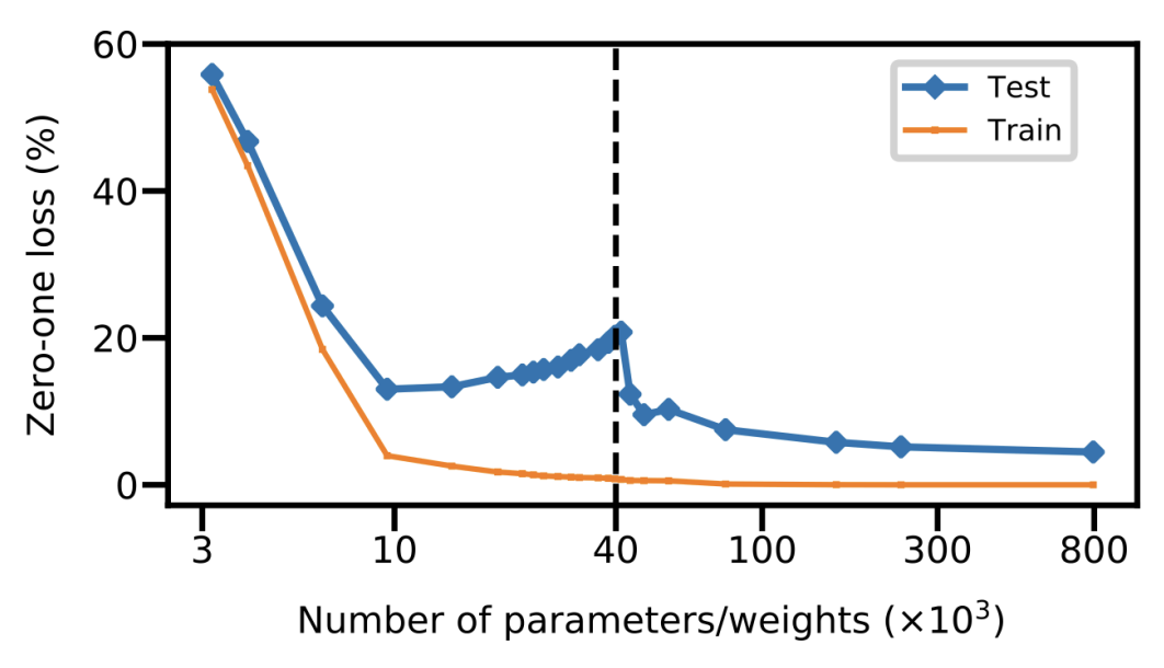
Here's a particular demonstration of double descent on the MNIST data set.

§ Implicit Regularization: Regression

This section aims to communicate the following vibe:

Vibe. The solution that gradient descent lands on will naturally tend to have small weights—even without a ridge penalty term!

We justify this vibe by demonstrating its validity specifically in the case of linear and logistic regression.

Theorem. (Linear Regression Implicit Regularization) Consider a linear regression $h \colon \mathbb{R}^d \to \mathbb{R}$ given by $h(x) := w^{\top}x$ with training error $\hat{\mathcal{R}}(w) := \|Xw - Y\|^2$ . Furthermore, assume that $d > n$ , meaning zero training error $\hat{\mathcal{R}}(w) = 0$ is achievable.

Among all parameters $w$ for which $\hat{\mathcal{R}}(w) = 0$ (or equivalently, $Xw = Y$ ), let $w^*$ denote the parameter with the lowest magnitude. Then GD with $w_0 = 0$ converges to $w^*$ .

Proof: As usual, let $X \in \mathbb{R}^{n \times d}$ and $Y \in \mathbb{R}^n$ encode the training data. Suppose GD with $w_0 = 0$ converges to $w_{\infty}$ .

Lemma 1. We have $w_{\infty} \in \mathrm{colspan}(X^{\top})$ .

Proof: Both $w_0 = 0$ and every update $\nabla \hat{\mathcal{R}}(w_t) \propto X^{\top}(Xw_t - Y)$ lie in $\mathrm{colspan}(X^{\top})$ . $\square$

Now consider any parameter $w$ for which $\hat{\mathcal{R}}(w) = 0$ (equivalently, $Xw = Y$ ). Since $\hat{\mathcal{R}}(w_{\infty}) = 0$ as well, we also have $Xw_{\infty} = Y$ . Therefore, if we denote $v := w - w_{\infty}$ , we have:

Xv = Xw - Xw_{\infty} = Y - Y = 0 ~ \implies ~ v \in \mathrm{ker}(X) = \mathrm{colspan}(X^{\top})^{\perp}.

In particular, since $w_{\infty} \in \mathrm{colspan}(X^{\top})$ by Lemma 1, this implies $\langle w_{\infty}, v \rangle = 0$ . Now the Pythagorean theorem gives $\|w\|^2 = \|w_{\infty}\|^2 + \|v\|^2 \geq \|w_{\infty}\|^2$ , with equality precisely when $w = w_{\infty}$ , as desired. $\blacksquare$

Remark. The exact same proof works just as well for SGD; all that changes is that the proof of Lemma 1 must specify that every possible update still lives in $\mathrm{colspan}(X^{\top})$ , which is easy to verify.

It turns out the same phenomenon can be proven true for logistic regression as well; proof omitted.

Theorem. (Logistic Regression Implicit Regularization) Given a linearly separable dataset, let $\mathcal{W}$ denote the set of all parameters $w$ such that $y_i \langle w, x_i \rangle \geq 1$ for all $i$ . Define $w^* := \argmin_{w \in \mathcal{W}} \|w\|^2$ .

Suppose we train a logistic regression on this dataset using GD with sufficiently small $\eta$ and any initialization $w_0$ . Then:

w_t = w^* \log t + O(\log \log t) ~ \text{ as } t \to \infty.

In particular, this implies that $\lim_{t \to \infty} \frac{w_t}{\|w_t\|} = \frac{w^*}{\|w^*\|}$ , so GD converges in the direction of $w^*$ .

§ Implicit Regularization: Early Stopping

It has also been observed that stopping training early can be a useful tactic for reducing testing error. For example, one might proceed with SGD until validation error increases.

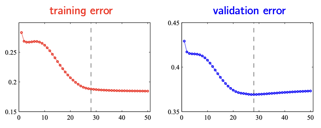
Informally, we can say the following; justification omitted.

Theorem. (Yao et al., 2007) For least squares regression, stopping GD early at time step $t$ is equivalent to ridge penalty $\frac{1}{\eta t} \|w\|^2$ .

Early stopping usually occurs before the interpolation threshold, meaning we stop before double descent becomes relevant.