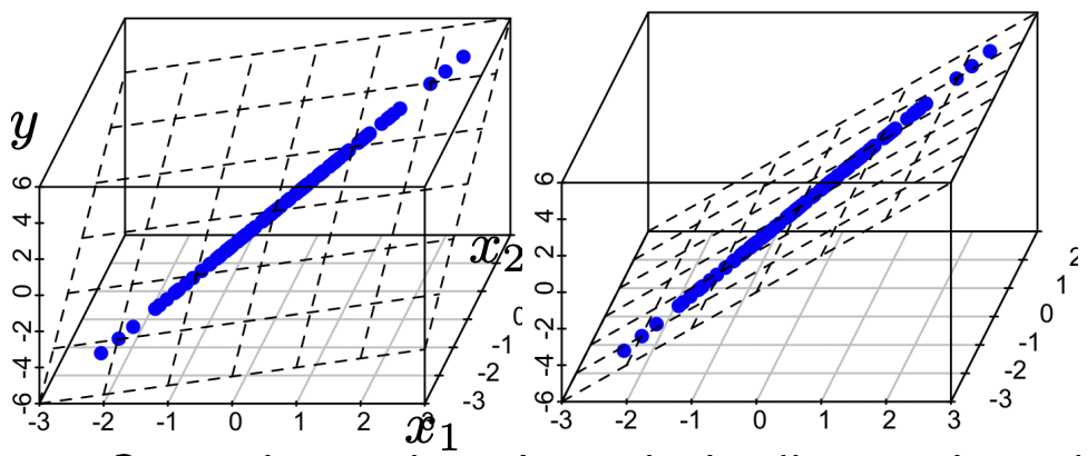
Recall that θ^=(X⊤X)−1X⊤Y is the minimizer of RSS(θ):=(Xθ−Y)⊤(Xθ−Y) (the “Residual Sum of Squares”). One possible problem is that X might not be full rank; two or more features might be perfectly collinear, making θ^ non-unique.
Maybe in practice, there's some tiny amount of noise in our observations, so X is “almost always” guaranteed to be full rank. That doesn't actually fix the issue at hand, though—the effect of that noise is still to effectively pick one of the infinitely-many maximum-likelihood choices for θ^ at random.
Remark. To clarify, collinearity of features isn't uncommon at all; take “credit card limit” and “credit card rating” as a practical example of two nearly-collinear features.
The issue is that linear regression is overconfident; it always returns a single point estimate θ^. Rather than decisively estimating the exact value of θ^, perhaps we should take a Bayesian approach: let incoming data {(x(n),y(n))}n=1Nupdate our priors on the distribution of θ instead.
§ Bayesian Linear Regression: Theory
Here's the model; refer to Lecture 21 of 18.650 for a reminder on Bayesian inference.
Our prior on θ is that θ∼N(μ0,Σ0), for arbitrary initial constants μ0 and Σ0.
We will assume that data (x(n),y(n)) is such that y(n)∼N(θ⊤x(n),σ2) for all n.
A prior and a model for our data are enough for us to determine the posteriors that result from reading in data.
Theorem. (Linear Regression Posterior) Suppose we collect N data points, represented by a matrix X and a column vector Y. Then the posterior is [θ∣X,Y]∼N(μN,ΣN), where μN and ΣN satisfy:
ΣN−1=Σ0−1+σ21X⊤X and ΣN−1μN=Σ0−1μ0+σ21X⊤Y
Remark. Goes without saying, but… even though these aren't explicit formulas for ΣN and μN, they do provide enough information to fully compute them if desired.
Proof: Plain computation, with some simplifying tricks. Recall that p(θ∣X,Y)∝p(θ)⋅LN(θ), where p(θ) is the PDF of a multivariable Gaussian, and LN(θ) is a product of N single-variable Gaussian PDFs.
p(θ)=(2π)Ddet(Σ0)1exp(−21(θ−μ0)⊤Σ0−1(θ−μ0)) and LN(θ)=(2πσ2)N1exp(−2σ21∥Y−Xθ∥2).
See Lecture 6 of 18.650 for a derivation of the multivariable case.
For ease of computation, it helps to instead work with logp(θ∣X,Y). Also recall that we only care about p(θ∣X,Y) up to a proportionality constant (as indicated by the ∝ symbol), so after taking logs, we can throw away any +C terms.
We'll compute the logarithm in two steps, starting with logp(θ). (Note that all terms in logp(θ) are real numbers.)
To arrive at line (★1), we absorbed the +μ0⊤Σ0−1μ0 into the +C because it is a real-number constant (i.e. has no θs).
To arrive at line (★2), we replaced θ⊤Σ0−1μ0 with μ0⊤Σ0−1θ. We can do this because they are real numbers and transposes of each other, so they are equal. In particular, (Σ0−1)⊤=Σ0−1 because covariance matrices Σ0 are symmetric.
Using some similar tricks, we can compute logLN(θ) as well.
We just need to compare this with the log of the PDF of N(μN,ΣN)… well, we already computed what the logarithm looks like—it's just line (★2) from earlier!
(♣2)log[PDF of N(μN,ΣN)]=θ⊤(−21ΣN−1)θ+(μN⊤ΣN−1)θ+C
Pattern-matching (♣1) against (♣2) (and taking the transpose of the latter equation…) yields the desired result. ■
Remark. The constant simplification of everything into the form θ⊤Aθ+bθ+c isn't a coincidence—every multivariable quadratic polynomial is expressible in such a form! See Lecture 16 of 18.701 for further detail.
§ Bayesian Linear Regression: Performance
The whole point of Bayesian linear regression is to avoid overconfidence. To what extent have we been successful?
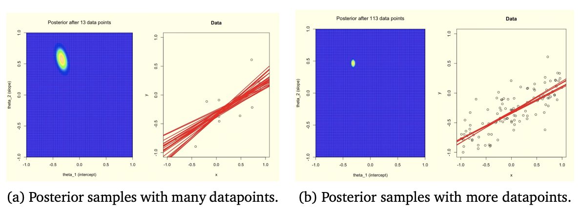
Example Set-Up. We draw features x(n)∼Unif[−1,1] and generate responses via y(n)∼N(θ1∗x(n)+θ0∗,σ2), where θ0∗=−0.3, θ1∗=0.5, and σ=0.2. The algorithm assumes the prior θ∼N(0,I2).
Under this set-up, Bayesian linear regression performs expectedly well; as more data comes in, the posterior becomes more focused around the correct value of θ.
But ordinary linear regression would do just as well here; there is no feature collinearity here.
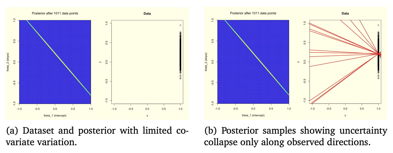
Altered Set-Up. Everything held constant, except the only feature value that is observed is x(n)=1.
This is equivalent to feature collinearity. (Recall that, for affine linear regression, all feature vectors have an extra “1” appended to their front to allow for “y-intercepts”; see Lecture 24 of 18.650.) Bayesian linear regression still performs well here!
The regression is able to be confident about θ∗ in some parameter directions, but not all parameter directions. There's still a one-dimensional space of potential values of θ∗=(θ0∗,θ1∗) that the regression sees as possible—still a strong improvement over the two-dimensional prior!
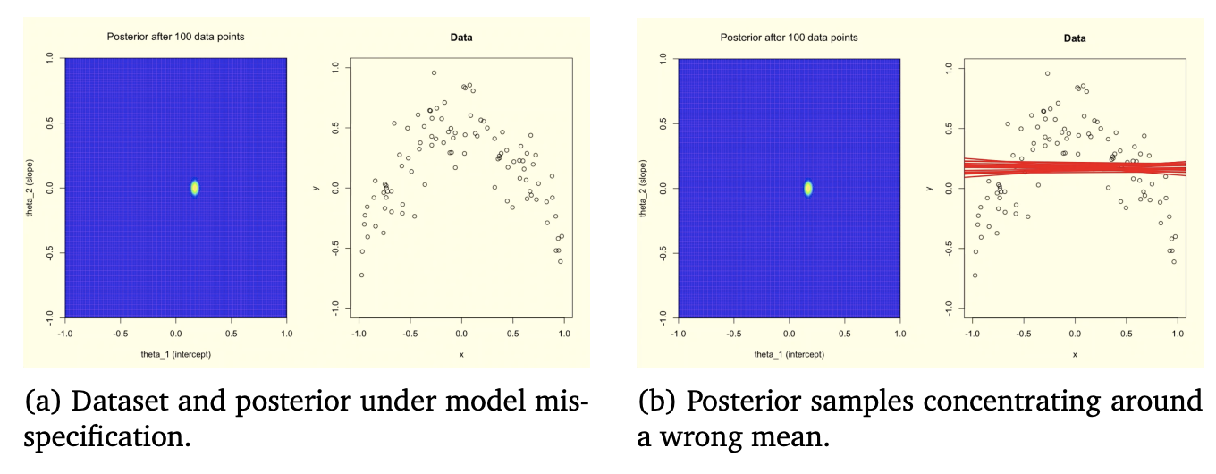
Further Altered Set-Up. The Bayesian regression believes responses are generated via y(n)∼N(θ1x(n)+θ0,σ2), but they're actually generated by y(n)∼N(0.5−(x(n))2,σ2).
Bayesian regression can't save you from model misspecification. As more data arrives, the posterior becomes more and more resolute in its estimate for θ, even though the regression hasn't come close to actually understanding the response generation.