MIT 6.790 — Lecture 6

Uncertainty, Regularizers, and Features

§ Aleatoric vs. Epistemic Uncertainty

There are two types of uncertainty that we would like to conceptually differentiate here.

Aleatoric Uncertainty. This refers to uncertainty caused by the intrinsic randomness in how the response $y^{(n)}$ relates to the feature vector $x^{(n)}$ . It's the uncertainty in the PDF $p(y \mid x, \theta)$ .

Epistemic Uncertainty. This refers to uncertainty caused by an incomplete model of the data being perceived. It's the uncertainty in the posterior $p(\theta \mid X, Y)$ caused by an insufficient amount of data.

Reading in more data will generally lessen the epistemic uncertainty, but more data won't be able to help with aleatoric uncertainty. As Lecture 5 showed, a misspecified model will produce great aleatoric uncertainty, yet the posterior overconfidently presents itself with very high epistemic certainty as it receives more data.

Remark. This overconfidence isn't unique to the Bayesian setting, of course; in the frequentist setting, standard errors and CI-widths also generally decrease as more data is read, even if the aleatoric uncertainty remains high.

§ MAP for Bayesian Linear Regression

We'll make some simplifying assumptions about our prior: assume $\theta \sim \mathcal{N}(0, \sigma_0^2 \cdot I_D)$ , where $D$ is the feature dimension. Then the posterior looks like the following; compare with the proof in Lecture 5, perhaps.

p(\theta \mid X, Y) \propto \underbrace{\mathrm{exp}\left( -\frac{\|Y - X\theta\|^2}{2\sigma^2} \right)}_{ \propto ~ L_N(\theta) } \cdot \underbrace{\mathrm{exp}\left( -\frac{\|\theta\|^2}{2\sigma_0^2} \right)}_{\propto ~ p(\theta)}.

Then the maximum a posteriori (MAP) satisfies the following:

Theorem. (Bayesian MAP) The maximum a posteriori for Bayesian linear regression, under the prior $\theta \sim \mathcal{N}(0, \sigma_0^2 I_D)$ , is:

\hat{\theta}_{\mathrm{MAP}} = \argmin_{\theta} \left[ \|X\theta - Y\|^2 + \frac{\sigma^2}{\sigma_0^2}\|\theta\|^2 \right] = \left(\frac{\sigma^2}{\sigma_0^2}I_D + X^{\top}X\right)^{-1} X^{\top}Y.

Proof: The first equality is trivial, so it remains to show the RHS expression for $\hat{\theta}_{\mathrm{MAP}}$ minimizes the middle expression. A shortcut is to just reuse the results we derived from Lecture 5, but for $(\mu_0, \Sigma_0) = (0, \sigma_0^2 I_D)$ .

\Sigma_N^{-1} = \frac{1}{\sigma_0^2} I_D + \frac{1}{\sigma^2} X^{\top}X ~~~ \text{ and } ~~~ \Sigma_N^{-1}\mu_N = \frac{1}{\sigma^2}X^{\top}Y.

The posterior distribution is a Gaussian $\mathcal{N}(\mu_N, \Sigma_N)$ , so it is maximized at $\hat{\theta}_{\mathrm{MAP}} = \mu_N$ . The result falls right out from there. $\blacksquare$

The quantity being minimized in the theorem statement above is referred to as the ridge regression objective.

It is the sum of our ordinary squared-loss and a new “ridge regression term”, the latter of which penalizes point estimates $\hat{\theta}_{\mathrm{MAP}}$ that have needlessly large coefficients—large coefficients in $\hat{\theta}_{\mathrm{MAP}}$ often suggest overfitting.

We'll oftentimes denote $\lambda := \frac{\sigma^2}{\sigma_0^2}$ in the ridge regression objective and expression for $\hat{\theta}_{\mathrm{MAP}}$ . Note that, while we can choose the value of $\sigma_0$ in our prior, we usually have no control or knowledge regarding $\sigma$ . So the value of $\lambda$ can alternatively be interpreted as a parameter of our choosing that indicates how strongly we want to discourage overfitting.

§ Features

Let's stop restricting ourselves to linear models. The idea is to create our own feature vectors whose entries are nonlinear functions of the entries of the feature vectors $\{x^{(n)}\}_{n = 1}^N$ .

Definition. We define our own features as $\phi: \mathbb{R}^D \to \mathbb{R}^P$ and write our regression hypothesis as $h(x) = \theta^{\top} \phi(x)$ .

Example. In the case of $D = 1$ , we might take $\phi(x) := \begin{bmatrix} 1 & x & x^2 \end{bmatrix}^{\top}$ , which yields the hypothesis $h(x) = \theta_0 + \theta_1x + \theta_2x^2$ .

Example. In the case of $D = 2$ , we might take $\phi(x) := \begin{bmatrix} 1 & x_1 & x_2 & x_1^2 & x_2^2 & x_1x_2 \end{bmatrix}^{\top}$ , and the set of all possible hypotheses becomes the set of all two-variable quadratic polynomials.

Here's how regression performs when we get nonlinear features involved.

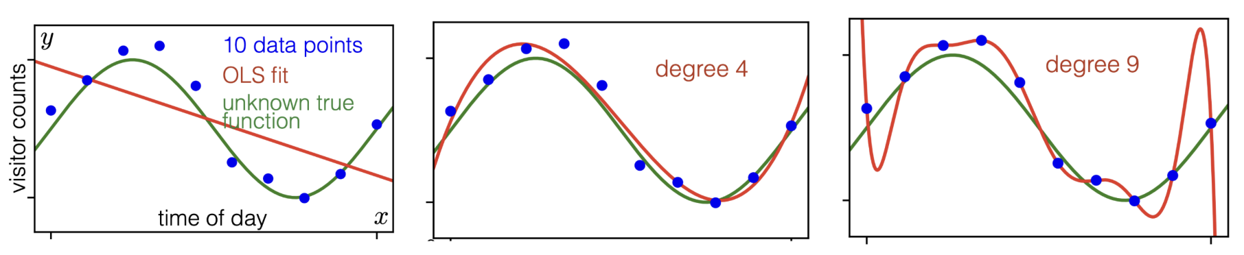
Notice how setting the feature dimension $P$ too large results in overfitting, to the point where our degree- $9$ regression is just performing Lagrange interpolation. To reduce overfitting, let's bring back a trick from just a few paragraphs ago: ridge regression.

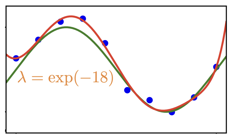
And so degree- $9$ regression works just fine with a ridge regression term using $\lambda = e^{-18}$ .

§ Kernel: Unlimited Features

There's another reason why too many features is bad: if we let $\Phi \in \mathbb{R}^{N \times P}$ (with rows $\phi(x^{(n)})^{\top}$ ) be our stand-in for $X \in \mathbb{R}^{N \times D}$ , then the ridge solution looks like:

\hat{\theta}_{\mathrm{MAP}} = \left( \lambda I_P + \Phi^{\top}\Phi \right)^{-1} \Phi^{\top}Y.

Computing this would require a $P \times P$ matrix inversion, which is far too computationally intensive for $P \gg D$ . So it seems like there is an upper bound on the number of features $P$ we can reasonably have.

Or maybe there isn't! We claim that there is an alternative way to approach our computation of ridge regressions that allows for $P$ to be arbitrarily large at no computational cost; the rest of this section is dedicated to showing how.

First, we claim the following theorem is true; the proof is unenlightening algebraic manipulation, so we omit it.

Theorem. (Bayesian MAP, Rewritten) The ridge solution $\hat{\theta}_{\mathrm{MAP}}$ may be expressed as:

\hat{\theta}_{\mathrm{MAP}} = \Phi^{\top}\left( \lambda I_N + \Phi\Phi^{\top} \right)^{-1}Y.

Note, importantly, that this implies that the ridge regression may be expressed as:

h(x) = \hat{\theta}^{\top}_{\mathrm{MAP}} \phi(x) = Y^{\top}\left( \lambda I_N + \Phi\Phi^{\top} \right)^{-1} \Phi \phi(x).

In this form, it turns out that there's a great amount of simplification to be made if we introduce the following:

Definition. The kernel is the function $k \colon \mathcal{X} \times \mathcal{X} \to \mathbb{R}$ (where $\mathcal{X}$ is the input space) given by $k(x^{(i)}, x^{(j)}) := \phi^{\top}(x^{(i)}) \phi(x^{(j)})$ .

Given data $\{x^{(n)}\}_{n = 1}^N$ , we may define a map $k: \mathcal{X} \to \mathbb{R}^N$ via $k(x)_i := k(x^{(i)}, x)$ . (Yes, overloaded notation.)
Given data $\{x^{(n)}\}_{n = 1}^N$ , we may define a matrix $K \in \mathbb{R}^{N \times N}$ given by $K_{i, j} := k(x^{(i)}, x^{(j)})$ .

We can now again rewrite the ridge regression formula using the language of the kernel.

Theorem. (Bayesian MAP, w/ Kernel) The ridge regression may be expressed as:

h(x) = Y^{\top}\left(\lambda I_N + K\right)^{-1} k(x).

Here's the upshot of all of this: the expression above only deals with matrices in $\mathbb{R}^{N \times N}$ and vectors in $\mathbb{R}^{N}$ ; there's no dependency on $P$ anywhere! So as long as we can efficiently compute the kernel $k \colon \mathcal{X} \times \mathcal{X} \to \mathbb{R}$ , we can set our number of features $P$ as large as we'd like.