MIT 6.790 — Lecture 9

Gradient Descent

§ Gradient Descent

Recall from Lecture 8 that logistic regression requires minimizing the following (logistic) loss:

\mathcal{L}(w) = \sum_{i = 1}^n \log_2\left[ 1 + \exp\left(-y^{(i)}w^{\top}x^{(i)}\right) \right].

Unfortunately, unlike with linear regression, there is no closed-form expression for the minimizing parameter of logistic loss. But because logistic loss is convex, we can apply gradient descent to find the global minimum. (Recall from Lecture 8 that we can say “global minimum” rather than “local minimum” because of convexity.)

Definition. Let $f \colon \mathbb{R}^n \to \mathbb{R}$ be a differentiable function. In gradient descent (GD), we start with some $w_0 \in \mathbb{R}^n$ and proceed via:

w_{t + 1} \leftarrow w_t - \eta \nabla f(w_t).

Note the hyperparameter $\eta > 0$ , which we call the step size. The hope is that $\{w_t\}_{t = 0}^{\infty}$ converges to a local minimizer of $f$ .

§ Stationary Points

Gradient descent stops at a value $w^* \in \mathbb{R}^n$ where $\nabla f(w^*) = 0$ ; we call such a point $w^*$ a stationary point. We can think of stationary points as being classifiable into two categories:

Category I: Global maximizers, global minimizers, local maximizers, or local minimizers.
Category II: Saddle points (as in, stationary points that are not Category I).

This is kind of irrelevant, though; gradient descent only converges to saddle points for a measure-zero set of initial points $w_0$ .

For a further discussion of how the Hessian relates to saddle points and whatnot, see Lecture 16 and Lecture 19 of 18.701 (specifically the subsections linked above).

§ Lower-Bounding GD Efficiency

For one-dimensional functions $f \colon \mathbb{R} \to \mathbb{R}$ , we can upper-bound the number of steps required to get close to a stationary point.

Theorem. (One-Dimensional Descent Lemma) Suppose $f \colon \mathbb{R} \to \mathbb{R}$ is twice differentiable, and $|f''(w)| \leq \beta$ for all $w$ . Then if we set $\eta = \frac{1}{\beta}$ , the iterates of gradient descent satisfy:

f(w_{t + 1}) - f(w_t) \leq -\frac{1}{2\beta} f'(w_t)^2.

In particular, each step of gradient descent produces an improvement of at least $\frac{1}{2\beta} f'(w_t)^2$ .

Proof: We won't provide a rigorous proof. The rough idea is to use the quadratic Taylor approximation.

f(w_{t + 1}) \approx f(w_t) + \delta f'(w_t) + \frac{\delta^2}{2}f''(w_t) ~ \text{ where } \delta = -\eta f'(w_t).

Plugging in $\delta = -\eta f'(w_t)$ and rearranging yields:

f(w_{t + 1}) - f(w_t) \approx - \eta f'(w_t)^2 \left[ 1 - \frac{\eta}{2} f''(w_t) \right] \leq -\frac{1}{2\beta} f'(w_t)^2 ~~~ \text{ assuming } \eta = \frac{1}{\beta} \text{ and } |f''(w)| \leq \beta.

That's the promised bound, with many computations omitted. This proof, of course, lacks rigor in that everything carries an $\approx$ symbol due to the Taylor approximation. $\blacksquare$

An immediate corollary of the Descent Lemma is the following.

Theorem. (One-Dimensional GD Efficiency) Suppose, in the setting of the Descent Lemma, that $f(w_0) - \min_w f(w) = M$ . If gradient descent yields $\{w_t\}_{t = 0}^{\infty}$ , then for any $\epsilon > 0$ , there is some $T \leq \frac{2 \beta M}{\epsilon^2}$ for which $|f'(w_T)| < \epsilon$ .

Remark. Note that none of the reasoning here carries an assumption that $f$ is convex.

For some reason, 6.790 does not state the multivariate versions of these theorems, even though their statements and proofs are nearly identical to the one-dimensional case. We state them here for completeness.

Theorem. (Multivariate Descent Lemma) Suppose $f \colon \mathbb{R}^n \to \mathbb{R}$ is twice differentiable, and $-\beta I \preceq \nabla^2 f(w) \preceq \beta I$ for all $w$ . Then if we set $\eta = \frac{1}{\beta}$ , the iterates of gradient descent satisfy:

f(w_{t + 1}) - f(w_t) \leq -\frac{1}{2\beta} \|\nabla f(w_t)\|^2.

In particular, each step of gradient descent produces an improvement of at least $\frac{1}{2\beta} \|\nabla f(w_t)\|^2$ .

Remark. The ordering $A \preceq B$ is the Loewner order on symmetric matrices: $A \preceq B$ if and only if $B - A$ is positive semidefinite.

Theorem. (Multivariate GD Efficiency) Suppose, in the setting of the Descent Lemma, that $f(w_0) - \min_w f(w) = M$ . If gradient descent yields $\{w_t\}_{t = 0}^{\infty}$ , then for any $\epsilon > 0$ , there is some $T \leq \frac{2 \beta M}{\epsilon^2}$ for which $\|\nabla f(w_T)\| < \epsilon$ .

§ Linear Regression Convergence Rate

Suppose we use gradient descent to find the minimum in simple least-squares linear regression. Then an overly large step size can cause gradient descent to fail to converge!

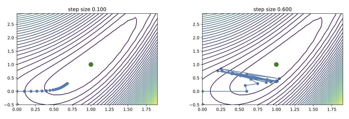
This often happens when the level sets of $f$ are elliptically-shaped, rather than spherically-shaped.

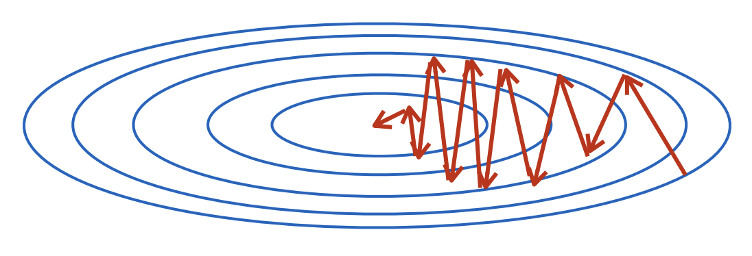
Let's investigate how this behavior appears specifically in the case of least-squares linear regression.

Theorem. (Least-Squares Gradient Descent) Suppose we use gradient descent to find a $w^* \in \mathbb{R}^d$ such that, given training data $X \in \mathbb{R}^{n \times d}$ and $y \in \mathbb{R}^n$ , the loss $f(w) := \|Xw - y\|^2$ is minimized. Then the sequence $\{w_t\}_{t = 0}^{\infty}$ satisfies:

w_t - w^* = (I_d - \eta H)^t (w_0 - w^*),

where $H := \nabla^2 f(w) = 2X^{\top}X$ is the Hessian matrix (notably, independent of $w$ ).

Proof: It's just plain computation. First, compute the relevant derivatives.

\nabla f(w) = 2X^{\top}(Xw - y) ~~~ \text{ and } ~~~ \nabla^2 f(w) = 2X^{\top}X.

Then note the minimizer $w^*$ is known to satisfy (see Lecture 23 of 18.650) the equation $X^{\top}Xw^* = X^{\top}y$ , so:

w_{t + 1} - w^* = \left[w_t - \underbrace{2 \eta \left( X^{\top}X w_t - X^{\top}y \right)}_{ = \ \eta \nabla f(w_t) }\right] - w^* = \left(I_d - 2 \eta X^{\top}X\right)(w_t - w^*).

Recalling $H = 2X^{\top}X$ and applying induction finishes the job. $\blacksquare$

For very large $t$ , the effect of $(I_d - \eta H)^t$ can be summarized by its eigenvalues. Say $\lambda_1 \geq \dots \geq \lambda_d > 0$ are the eigenvalues of $H$ . Then we can make the following observations.

The eigenvalues of $I_d - \eta H$ are precisely $\left\{1 - \eta \lambda_i\right\}_{i = 1}^d$ .
To ensure convergence, we require all eigenvalues to be in $(-1, 1)$ .
- The largest eigenvalue $\lambda_1$ gives the tightest bound here; the constraint $1 - \eta \lambda_1 \in (-1, 1)$ implies $\eta \lesssim \frac{1}{\lambda_1}$ , roughly.
However, smaller values of $\eta$ lead to slower convergence, as $1 - \eta \lambda_i$ is further from $0$ when $\eta$ is smaller.
- The smallest eigenvalue $\lambda_d$ gives the slowest convergence here. For $\eta = \frac{1}{\lambda_1}$ , the decay is:
  $\|w_t - w^*\|^2 \leq \left(1 - \frac{\lambda_d}{\lambda_1}\right)^{2t} \|w_0 - w^*\|^2.$

We can summarize this whole story like so.

Definition. Let the condition number $\kappa$ of a matrix $H$ be $\kappa := \frac{\lambda_{\mathrm{max}}(H)}{\lambda_{\mathrm{min}}(H)}$ (the ratio of its largest eigenvalue to its smallest).

Theorem. (Least-Squares Convergence Rate) Gradient descent for least-squares linear regression, with step size $\eta = \frac{1}{\lambda_{\mathrm{max}}(H)}$ , converges to the global minimum at an exponential rate, described below.

\|w_t - w^*\|^2 \leq \left(1 - \frac{1}{\kappa}\right)^{2t} \|w_0 - w^*\|^2.

This also explains why elliptically-shaped level sets yield slower convergence: they have a larger condition number.