MIT 6.790 — Lecture 13

Neural Networks: Depth and Optimization

§ Neural Network Depth

In this section, we provide an example of a deep ReLU-activated network that cannot be accurately represented by a shallow ReLU-activated network (without using an excessive number of nodes). Formally, we show:

Theorem. (Depth Necessity) For every $L \in \mathbb{N}$ , we can construct a function $f \colon [0, 1] \to [0, 1]$ such that:

It is exactly representable by a ReLU network of depth $O(L^2)$ with $O(L^2)$ nodes.
For any ReLU network $h \colon [0, 1] \to \mathbb{R}$ of depth $L$ with at most $2^L$ nodes, we have $\int_{0}^1 |f(x) - h(x)| \, \mathrm{d}x \geq \frac{1}{8}$ .

Remark. As a reminder, the ReLU activation function is $\mathrm{ReLU}(t) := \max(t, 0)$ .

To prove this theorem, we'll need the following lemma.

Theorem. (ReLU Breakpoints) If $h \colon \mathbb{R} \to \mathbb{R}$ is a ReLU network with hidden layer widths $m_1, m_2, \dots, m_L$ , then $h$ is a piecewise linear function with at most $2^{L - 1} (m_1 + 1)m_2 \dots m_L$ linear pieces.

Proof: Induction on $L$ . The base case of $L = 1$ states that a linear combination of $m$ ReLUs is piecewise linear with at most $m + 1$ linear pieces, which is obviously true.

For the inductive step, the point is the following:

Claim. Passing a piecewise linear function with $T$ linear pieces through a ReLU at most doubles the number of linear pieces.

Justification: Each linear piece either stays a single piece or gets split in two, depending on if it crosses the $x$ -axis.

Each pre-activation in the $L^{\text{th}}$ hidden layer is the output of a ReLU network with $L - 1$ layers and hidden layer widths $m_1, m_2, \dots, m_{L - 1}$ . Thus, each $L^{\text{th}}$ -layer pre-activation has at most $N := 2^{L - 2}(m_1 + 1)m_2\dots m_{L - 1}$ linear pieces by the inductive hypothesis.

Then the claim above implies that each $L^{\text{th}}$ -layer neuron has at most $2N$ linear pieces. And the final output is a linear combination of $m_L$ such neurons, hence an upper bound of $2Nm_L = 2^{L - 1}(m_1 + 1)m_2\dots m_L$ , as desired. $\blacksquare$

Now for the proof of the “Depth Necessity” theorem from earlier.

Proof: Consider the tent map $\tau \colon [0, 1] \to [0, 1]$ given by:

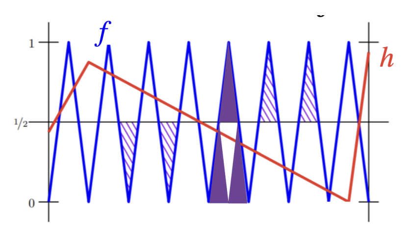
\tau(x) := 2 \cdot \left[\mathrm{ReLU}(x) - \mathrm{ReLU}(2x - 1)\right] = \begin{cases} 2x & x \leq \frac{1}{2}. \\ 2 - 2x & x > \frac{1}{2}. \end{cases}

Then a depth- $O(L^2)$ network can produce the function $f(x) := \tau^{(\circ) L^2}(x)$ (that is, $\tau$ composed with itself $L^2$ times). The result is a function with $2^{L^2 - 1}$ oscillations; here's how $f(x)$ looks for $L = 2$ , for example.

Any output $h \colon [0, 1] \to \mathbb{R}$ of a ReLU network of depth $L$ and at most $2^L$ nodes has (according to the previous theorem):

\text{\# of linear pieces} \leq 2^{L - 1} \cdot \left[(m_1 + 1)m_2 \dots m_L\right] \leq 2^{L - 1} \cdot \left[\frac{2^L}{L}\right]^{L} \leq 2^{L^2 - 1}.

We used some very crude estimates here, including an AM-GM bound.

The point is that $f(x)$ forms $2^{L^2}$ triangles with the line $y = \frac{1}{2}$ (see the diagram above). But $h$ can only change direction at most $2^{L^2 - 1}$ times, so $h$ must be on the “wrong side” of at least half of the triangles.

And the integral of $|f(x) - h(x)|$ over just the intervals where $h$ is on the “wrong side” is already $\frac{1}{8}$ , as desired. $\blacksquare$

Remark. Some of our bounds here are really loose, enough so that the $\frac{1}{8}$ bound doesn't fully hold water as presented. But the holes are easy to fix if we settle for a smaller constant, say; the gist of the proof is still fully present.

§ Neural Network Optimization

Neural networks are a parametric model with parameters $\theta := \{W^{(i)}, b^{(i)}\}_{i = 1}^{L + 1}$ . As with any parametric model, we tune the parameter $\theta$ by minimizing the empirical risk (ERM). Specifically, we assume the following:

Our loss function is $\mathcal{L}\left(h_{\theta}(x^{(t)}), y^{(t)}\right) := \left(h_{\theta}(x^{(t)}) - y^{(t)}\right)^2$ (that is, squared loss).
We employ a variant of (stochastic) gradient descent: for each training example $(x^{(t)}, y^{(t)})$ , we perform the update:
$\theta' \gets \theta - \alpha \cdot \nabla_{\theta} \left[ \mathcal{L}\left(h_{\theta}(x^{(t)}), y^{(t)}\right) + \lambda \cdot \Omega(\theta) \right].$
Here, $\alpha$ and $\lambda$ are hyperparameters, and $\Omega(\theta) := \sum_{i = 1}^{L + 1} \|W^{(i)}\|^2_F$ is a Frobenius regularizer.
- Note that $\|M\|^2_F$ denotes the sum of the squares of all of the entries in $M$ .
- Recall from Lecture 6 that regularizers (e.g. ridge regression terms) penalize large parameters to discourage overfitting.

The gradient of the regularizer is easy to compute—the gradient of $\mathcal{L}(h_{\theta}(x), y)$ , less so.

§ Chain Rule Warm-Up

The rest of this lecture is dedicated to the computation of the gradient of $\mathcal{L}(h_{\theta}(x), y)$ . First, a chain rule warm-up.

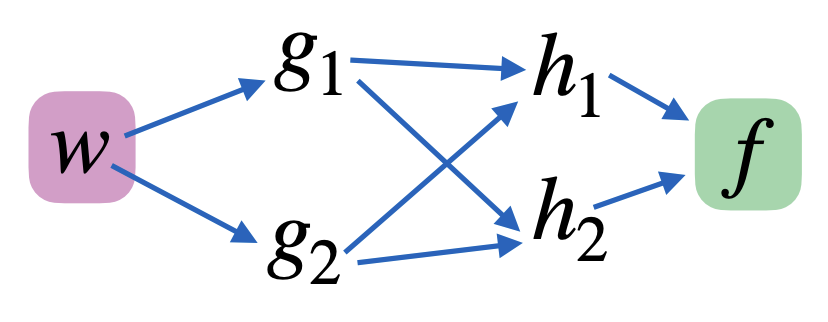
Problem. Write an expression for $\frac{\partial f}{\partial w}$ given the computational graph shown below.

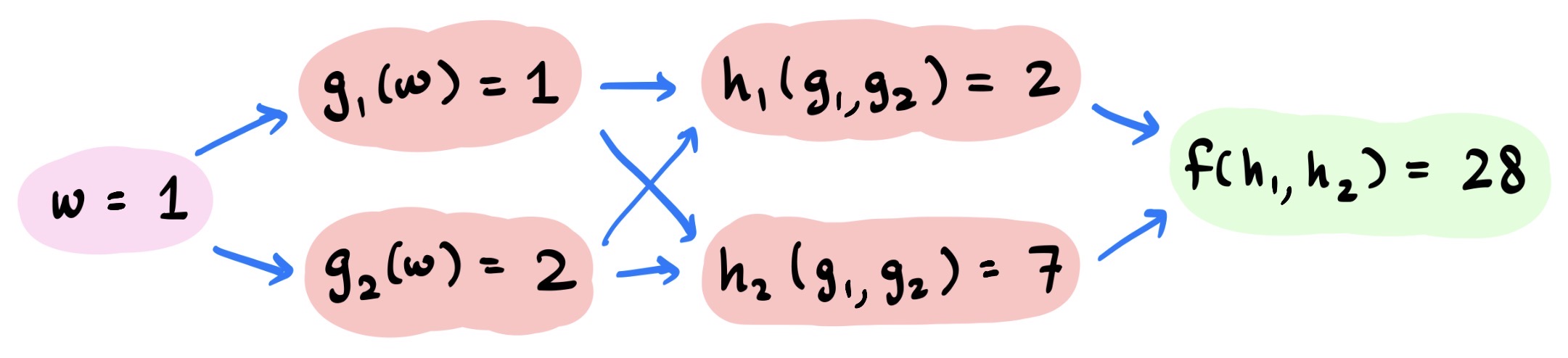
Solution: There is one term for each of the four paths from $w$ to $f$ in the graph; each term is the product of all of the partial derivatives along that path.

\frac{\partial f}{\partial w} = \left[ \frac{\partial f}{\partial h_1} \frac{\partial h_1}{\partial g_1} \frac{\partial g_1}{\partial w} \right] + \left[ \frac{\partial f}{\partial h_1} \frac{\partial h_1}{\partial g_2} \frac{\partial g_2}{\partial w} \right] + \left[ \frac{\partial f}{\partial h_2} \frac{\partial h_2}{\partial g_1} \frac{\partial g_1}{\partial w} \right] + \left[ \frac{\partial f}{\partial h_2} \frac{\partial h_2}{\partial g_2} \frac{\partial g_2}{\partial w} \right].

To help concretize this symbol slop, let's actually compute this partial derivative given the following functions:

g_1(w) = 3w - 2 ~~~ \parallel ~~~ g_2(w) = w^2 + 1 ~~~ \parallel ~~~ h_1(g_1, g_2) = g_1g_2 ~~~ \parallel ~~~ h_2(g_1, g_2) = g_2^3 - g_1^2 ~~~ \parallel ~~~ f(h_1, h_2) = h_1^2h_2

Let's compute $\frac{\partial f}{\partial w}$ when $w = 1$ . The first step is a forward pass: compute every function at $w = 1$ .

Separately, we may compute all of the partial derivatives:

\frac{\partial g_1}{\partial w} = 3 ~~ \parallel ~~ \frac{\partial g_2}{\partial w} = 2w ~~ \parallel ~~ \frac{\partial h_1}{\partial g_1} = g_2 ~~ \parallel ~~ \frac{\partial h_1}{\partial g_2} = g_1 ~~ \parallel ~~ \frac{\partial h_2}{\partial g_1} = -2g_1 ~~ \parallel ~~ \frac{\partial h_2}{\partial g_2} = 3g_2^2 ~~ \parallel ~~ \frac{\partial f}{\partial h_1} = 2h_1h_2 ~~ \parallel ~~ \frac{\partial f}{\partial h_2} = h_1^2

Notice that most of these expressions are not direct functions of $w$ . In order to evaluate them at $w = 1$ , we must have done the precomputation of every function's value at $w = 1$ via a forward pass.

Here's how it would look to compute the second of the four terms in $\frac{\partial f}{\partial w}$ .

\frac{\partial f}{\partial h_1} \times \frac{\partial h_1}{\partial g_2} \times \frac{\partial g_2}{\partial w} = 2(h_1)(h_2) \times g_1 \times 2w = 2(2)(7) \times (1) \times 2(1) = \boxed{56}.

If we were to carry out the full computations for $\frac{\partial f}{\partial w}$ , we would have to compute:

All $6$ node values in the graph. (The forward pass.)
All $8$ partial derivative functions, and all $8$ of their evaluations at $w = 1$ .
A total of $8$ multiplications of partial derivatives and $3$ additions of products of partial derivatives.

§ Neuron Warm-Up

Again, as a warm-up, we'll start by investigating the gradients in the simplest possible neural network.

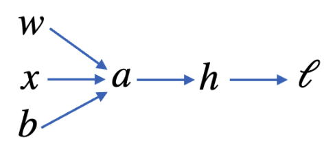
Warm-Up. In a single-neuron one-dimensional neural network, here's how $\nabla_{\theta} \mathcal{L}(h_{\theta}(x), y)$ is computed.

Here, the pre-activation is $a \colon \mathbb{R} \to \mathbb{R}$ via $a(x) = b + wx$ , and the activation is $h(x) := g(a(x))$ . We follow the same approach as before; first calculate each node's value via a forward pass, then compute:

\frac{\partial \mathcal{L}}{\partial w} = \frac{\partial \mathcal{L}}{\partial h} \cdot \frac{\partial h}{\partial a} \cdot \frac{\partial a}{\partial w} = 2(h(x) - y) \cdot g'(a(x)) \cdot x ~~~ \parallel ~~~ \frac{\partial \mathcal{L}}{\partial b} = \frac{\partial \mathcal{L}}{\partial h} \cdot \frac{\partial h}{\partial a} \cdot \frac{\partial a}{\partial b} = 2(h(x) - y) \cdot g'(a(x)) \cdot 1

Note that there is only one path from $w$ to $\mathcal{L}$ (as well as from $b$ to $\mathcal{L}$ ), so there are no sums yet.

§ Backpropagation Example

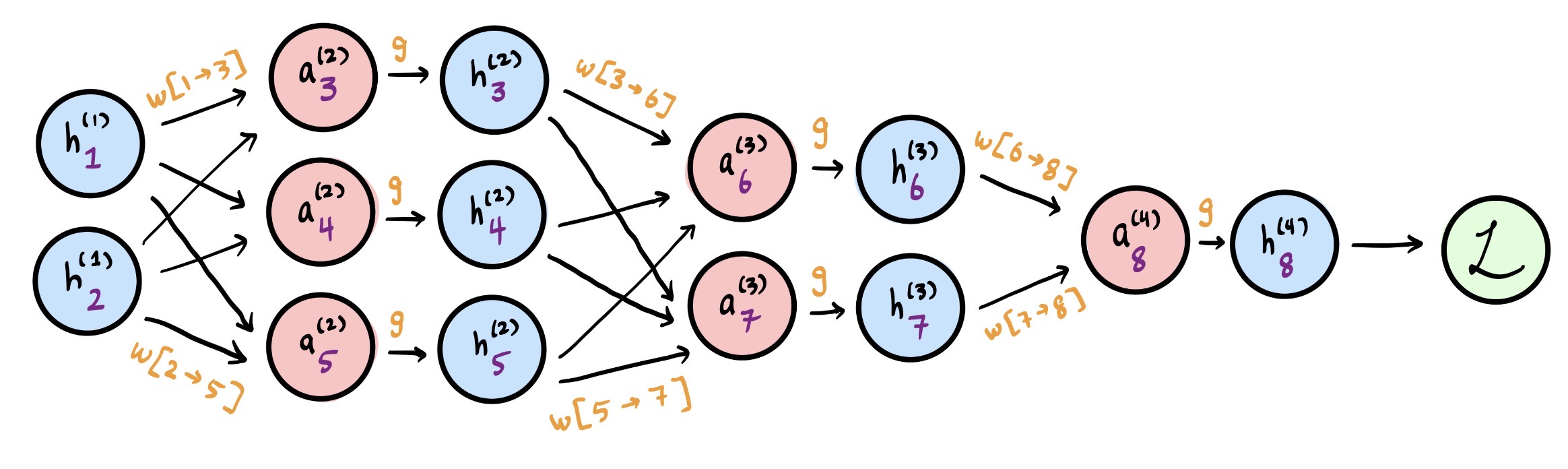
Now suppose we have several layers, each with several neurons. We don't draw out each of the parameters $\{(W^{(i)}, b^{(i)})\}_{i = 1}^{L + 1}$ as input nodes to each pre-activation $a^{(i)}$ , though. Instead, the drawing below shows the following:

The only nodes are the $\mathbb{R}$ -valued pre-activations $a^{(i)}$ and their activations $h^{(i)}$ .
Each pre-activation and its corresponding activation is given a unique index, written as a purple subscript.
For each entry of each matrix $W^{(i)}$ , that entry represents the weight of a directed edge from an activation $h^{(i - 1)}_u$ to a pre-activation $a^{(i)}_v$ . That weight is hence denoted $w[u \to v]$ .
We ignore the biases $\{b^{(i)}\}_{i = 1}^{L + 1}$ for now, though they operate almost identically.

Importantly, each $w[u \to v]$ edge is an input to the pre-activation it feeds into; the variable $w[u \to v]$ just doesn't get a node.

Remark. The diagram above makes a minor mistake—the superscripts should read $\{(0), (1), (2), (3)\}$ , as the leftmost layer shown is the input layer, not a hidden layer.

Our ultimate goal is to compute $\frac{\partial \mathcal{L}}{\partial w[u \to v]}$ for all edges $w[u \to v]$ in the network. However, notice the following:

\frac{\partial \mathcal{L}}{\partial w[u \to v]} = \frac{\partial \mathcal{L}}{\partial a_v} \cdot \frac{\partial a_v}{\partial w[u \to v]} = \frac{\partial \mathcal{L}}{\partial a_v} \cdot h_u.

It's easy to compute all values of $h_u$ via a forward pass; it remains to compute $\delta[v] := \frac{\partial \mathcal{L}}{\partial a_v}$ for all $v$ .

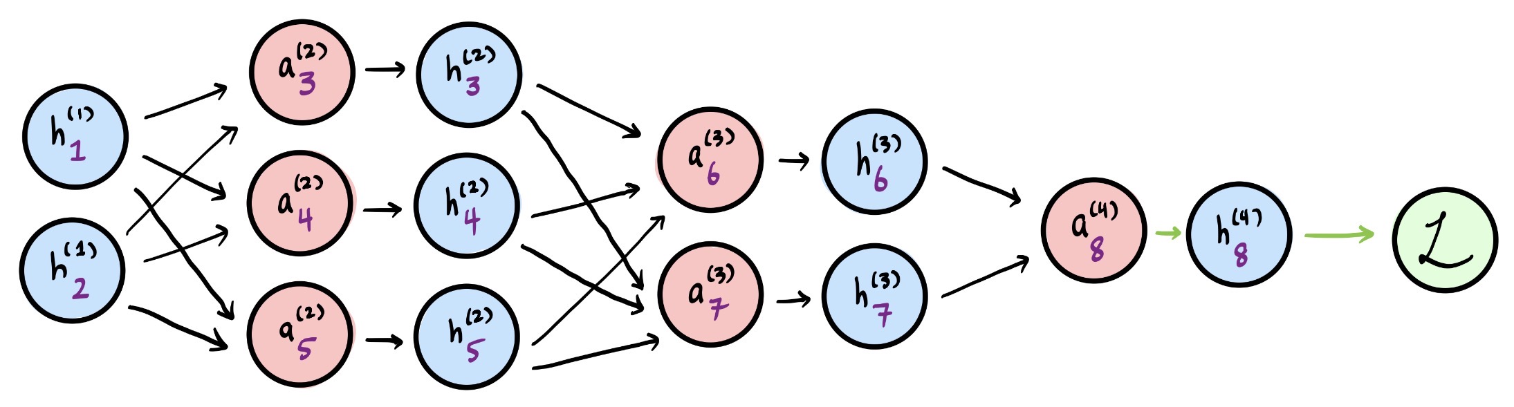
This is the backward pass, done via an induction-flavored approach. The “base case” is $\delta[8]$ , the pre-activation node closest to $\mathcal{L}$ .

The green arrows show the only path from $a_8$ to $\mathcal{L}$ ; in general, the base case will only have one such path. This yields:

\delta[8] = \frac{\partial \mathcal{L}}{\partial a_8} = \frac{\partial \mathcal{L}}{\partial h_8} \cdot \frac{\partial h_8}{\partial a_8} = 2(h_8 - y) \cdot g'(a_8).

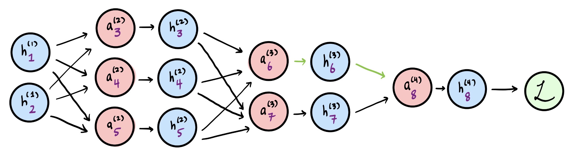
Now, if we wish to compute $\delta[6]$ , the trick is to use our newfound knowledge of $\delta[8]$ .

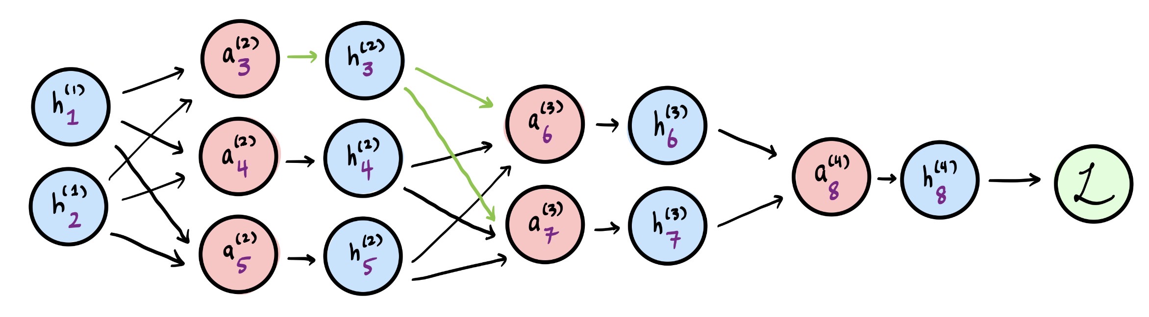
By propagating backwards, we minimize computational redundancies by computing earlier values of $\delta$ in terms of later ones.

\delta[6] = \frac{\partial \mathcal{L}}{\partial a_6} = \frac{\partial \mathcal{L}}{\partial a_8} \cdot \frac{\partial a_8}{\partial h_6} \cdot \frac{\partial h_6}{\partial a_6} = \delta[8] \cdot w[6 \to 8] \cdot g'(a_6).

We can compute $\delta[7]$ in the same way. With that layer complete, we now move back a layer and tackle $\delta[3]$ .

In this case, there are two paths from $a_3$ to the $3^{\text{rd}}$ layer, so our derivative has two terms.

\delta[3] = \frac{\partial \mathcal{L}}{\partial a_3} = \left[ \frac{\partial \mathcal{L}}{\partial a_6} \cdot \frac{\partial a_6}{\partial h_3} \cdot \frac{\partial h_3}{\partial a_3} \right] + \left[ \frac{\partial \mathcal{L}}{\partial a_7} \cdot \frac{\partial a_7}{\partial h_3} \cdot \frac{\partial h_3}{\partial a_3} \right] = g'(a_3) \cdot \left[ \delta[6] \cdot w[3 \to 6] + \delta[7] \cdot w[3 \to 7] \right].

And we can compute $\delta[4]$ and $\delta[5]$ in the exact same way.

§ Backpropagation Statement

Using the notation established in the previous example, we can now describe the backpropagation algorithm.

Backpropagation. After reading in a training example $(x, y)$ …

First, perform a forward pass: precompute $h_i(x)$ and $g'(a_i(x))$ for every activation $h_i$ and pre-activation $a_i$ in the NN.
Next, the backward pass: compute $\delta[u] := \frac{\partial \mathcal{L}}{\partial a_u}$ for every pre-activation $a_u$ as follows.
- Say the output layer has pre-activation $a_F$ . Then $\delta[F] = 2(h_F(x) - y) \cdot g'(a_F)$ .
- For the rest, compute $\delta[u]$ inductively via $\delta[u] = g'(a_u) \cdot \left[ \sum_{v \colon u \to v} \delta[v] \cdot w[u \to v] \right]$ .
Update the parameters $\{(W^{(i)}, b^{(i)})\}_{i = 1}^{L + 1}$ like so:
$w[u \to v] \gets w[u \to v] - \alpha \cdot \delta[v] \cdot h_u(x) ~~~ \parallel ~~~ b[v] \gets b[v] - \alpha \cdot \delta[v].$

(You can check for yourself that the updating formula for $b[v]$ is also correct.)