MIT 6.790 — Lecture 11

PAC and VC Dimension

§ Probably Approximately Correct (PAC)

The result from the end of Lecture 10 inspires the following definition.

Definition. For $\epsilon > 0$ and $\delta \in (0, 1)$ , a learning algorithm that takes training data $\mathcal{D}$ and outputs a hypothesis $\hat{h}$ is $(\epsilon, \delta)$ -PAC if:

\mathbb{P}\left( \mathcal{R}(\hat{h}) - \mathcal{R}(h^*) \leq \epsilon \right) \geq 1 - \delta,

where, as before, we denote $h^* := \argmin_{h \in \mathcal{H}} \mathcal{R}(h)$ .

Think of $\epsilon$ as an accuracy parameter that represents the difference between the learned and optimal hypotheses $\hat{h}$ and $h^*$ .
Think of $\delta$ as a confidence parameter that represents the chance that our data $\mathcal{D}$ misrepresents the actual data distribution.

Example. The result from Lecture 10 says that, if the risk function $\mathcal{R}(h)$ has a loss function satisfying $\mathcal{L}(x, y) \in [0, 1]$ , then the ERM learning algorithm is $\left(2 \sqrt{\frac{\log |\mathcal{H}| + \log\left(2 / \delta\right)}{2|\mathcal{D}|}}, \delta \right)$ -PAC.

§ PAC-Learnable

Definition. A hypothesis class $\mathcal{H}$ is PAC-learnable if there exists a learning algorithm that takes training data $\mathcal{D}$ and outputs a hypothesis $\hat{h}$ such that the following is true for any $\epsilon > 0$ and $\delta \in (0, 1)$ .

There exists a constant $m_{\mathcal{H}}(\epsilon, \delta)$ such that, no matter what the data distribution, $\hat{h}$ is $(\epsilon, \delta)$ -PAC whenever $|\mathcal{D}| > m_{\mathcal{H}}(\epsilon, \delta)$ .

Example. The result from Lecture 10 says that any finite hypothesis class $\mathcal{H}$ is PAC-learnable (assuming a bounded loss function). In particular, in this case we have $m_{\mathcal{H}} = O\left( \frac{\log|\mathcal{H}| + \log(1/\delta)}{\epsilon^2} \right)$ .

The assumption of “bounded loss” in the above example actually turns out to be pretty much required.

Fact. If the loss function is unbounded, then it turns out almost nothing is PAC-learnable.

Justification: Let's consider the simplest nontrivial case: $\mathcal{H} = \{h_1, h_2\}$ . Then consider the following distribution on $\mathcal{D}$ .

(a)
With very small probability $p$ , we sample $(x, y)$ for which $\mathcal{L}(h_1(x), y) = M$ and $\mathcal{L}(h_2(x), y) = 1$ , where $M \gg 1$ .
(b)
With very large probability $1 - p$ , we sample $(x, y)$ for which $\mathcal{L}(h_1(x), y) = \mathcal{L}(h_2(x), y)$ .

Then no matter how large an $m_{\mathcal{H}}(\epsilon, \delta)$ we pick, we can set $p$ small enough so that $\mathcal{D}$ almost always hits case (b). Then it is impossible for the learning algorithm to learn that $h_2$ is the better hypothesis.

Thematically, the reason why unbounded loss leads to PAC-unlearnability is that unbounded nonnegative random variables can have means that are impossible to bound given only finitely many samples.

The conclusion, then, is that we might as well assume the loss function is bounded. We should also direct our attention to infinite hypothesis classes $\mathcal{H}$ , as all the finite ones are automatically PAC-learnable under this assumption.

§ Growth Functions: Motivation

From now on, we'll specifically consider the case when our hypotheses $h \in \mathcal{H}$ are binary classifiers $h \colon \mathcal{X} \to \{+1, -1\}$ . Even still, proving or disproving PAC-learnability for infinite hypothesis classes seems hard.

Remark. This subsection and the next will take a step back from PAC-learnability for a while. Just have trust that all of this setup will eventually prove itself incredibly useful for deciding whether an infinite hypothesis class is PAC-learnable or not.

Suppose $m$ is the size of our training data $\mathcal{D} = \{(x_i, y_i)\}_{i = 1}^m$ . Then there are only so many ways a hypothesis $h \in \mathcal{H}$ can perform in the training process. The training data acts like an $m$ -question true-or-false exam, so there are at most $2^m$ ways a hypothesis $h \in \mathcal{H}$ could perform. Our learning algorithm should pick the hypothesis $\hat{h} \in \mathcal{H}$ that scores the highest.

But if two hypotheses $\{h_1, h_2\}$ score the highest… well, then we haven't learned enough. It's possible that our learning algorithm outputs $\hat{h} = h_1$ , whereas the true optimal hypothesis is $h^* = h_2$ . And maybe on the real test data, the output $\hat{h}$ performs horribly in comparison to $h^*$ . We'd have no way of knowing, because $\hat{h}$ and $h^*$ performed the same in the training exam.

§ Growth Functions: Definition

To formalize the idea of multiple hypotheses ending up indistinguishable in training, it helps to count the number of possible ways a hypothesis $h \in \mathcal{H}$ can perform on our $m$ -question true-or-false exam.

Definition. Given a training set $X = (x^{(1)}, \dots, x^{(m)}) \in \mathcal{X}^m$ , let $\mathcal{H}_X$ denote the set of all possible labelings of points in $X$ by some hypothesis in $\mathcal{H}$ ; that is,

\mathcal{H}_X := \left\{ \left(h(x^{(1)}), \dots, h(x^{(m)})\right) \mid h \in \mathcal{H} \right\}.

Definition. Define $\Gamma_{\mathcal{H}}(m) := \displaystyle \max_{X \in \mathcal{X}^m} |\mathcal{H}_X|$ to be the growth function of $\mathcal{H}$ .

Example. In the worst case, we have $\Gamma_{\mathcal{H}}(m) = 2^m$ for all $m$ . This represents the scenario in which multiple hypotheses are the highest-scoring, making it impossible to pick out a PAC hypothesis.

Remark. By definition, $\Gamma_{\mathcal{H}}(m) > 2^m$ is impossible.

Problem. Determine the growth function of $\mathcal{H} := \{x \mapsto \mathrm{sgn}(x - \theta) \mid \theta \in \mathbb{R}\}$ .

Solution: Suppose the training set is $x^{(1)} < \dots < x^{(m)}$ , in that order. Then there are only $\Gamma_{\mathcal{H}}(m) = \boxed{m + 1}$ ways a hypothesis in $\mathcal{H}$ could label these points; one such way is pictured below.

Problem. Let $\mathcal{H}$ be the class of all two-dimensional linear classifiers. Compute $\Gamma_{\mathcal{H}}(3)$ and $\Gamma_{\mathcal{H}}(4)$ .

Solution: The picture below demonstrates that $\Gamma_{\mathcal{H}}(3) = \boxed{8}$ and is achieved by any three points in general position.

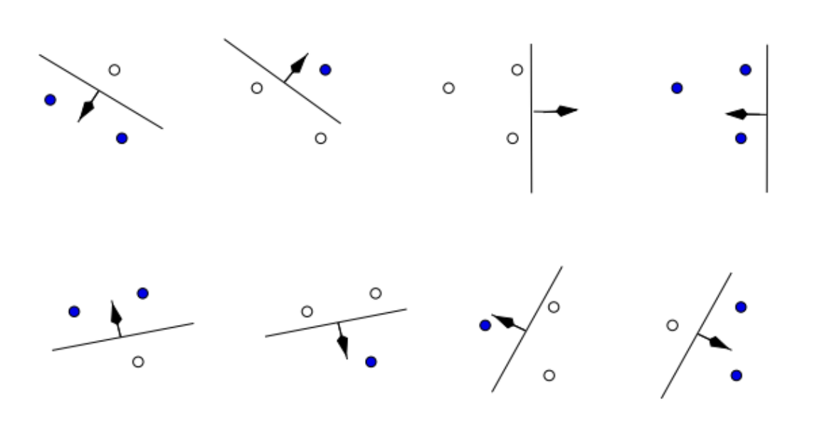
Interestingly, $\Gamma_{\mathcal{H}}(4)$ does not equal $2^4 = 16$ . If the four points of our data set are taken to be the vertices of a square, then not all $2^4$ labelings of those vertices are achievable by a linear classifier.

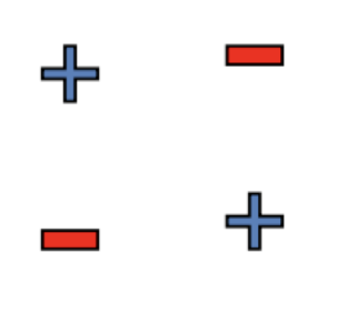
Infamously, as shown above, the XOR cannot be modeled by a linear classifier, and $\Gamma_{\mathcal{H}}(4) = \boxed{14}$ instead of $16$ . (To prove this, we would have to check that no other arrangement of four points gives more than $14$ achievable labelings.)

§ VC Dimension

Shockingly, as the following theorem states, there are only two types of growth functions.

Theorem. (VC Dichotomy) For any hypothesis class $\mathcal{H}$ , either:

We have $\Gamma_{\mathcal{H}}(N) = 2^N$ for all $N$ .
We have $\Gamma_{\mathcal{H}}(N) \leq C \cdot N^d$ for all $N$ , for some constants $C > 0$ and $d \in \mathbb{N}$ .

Remark. Note that this theorem is fundamentally a set-theoretic result! Nothing about its statement requires any mention of a probability distribution or machine learning at all.

This inspires the following definitions.

Definition. A training set $X \in \mathcal{X}^m$ is shattered by a hypothesis class $\mathcal{H}$ if $|\mathcal{H}_X| = 2^m$ . The VC-dimension $\mathrm{VC}(\mathcal{H})$ of a hypothesis class $\mathcal{H}$ is the size of the largest subset of $\mathcal{X}$ that is shattered by $\mathcal{H}$ .

Example. If $\mathcal{H}$ is such that $\Gamma_{\mathcal{H}}(N) = 2^N$ for all $N$ , then its VC-dimension is infinite. Meanwhile,

The VC-dimension of the hypothesis class $\mathcal{H} := \{x \mapsto \mathrm{sgn}(x - \theta) \mid \theta \in \mathbb{R}\}$ from earlier is $1$ .
The VC-dimension of the class of all two-dimensional linear classifiers is $3$ .
More generally, you can check that the VC-dimension of the class of all $d$ -dimensional linear classifiers is $d + 1$ .

Remark. You might notice that the VC-dimension of each of these examples happens to equal the number of parameters associated with its hypothesis class. Please note that this does not hold in general.

§ Results: Identifying PAC-Learnability

Now we can finally get back to PAC-learnability! Let's state (without proof) some results using our newfound definitions.

Theorem. (ERM VC Risk Bound) Under the ERM learning algorithm, the following holds with probability at least $1 - \delta$ .

\mathcal{R}(\hat{h}) \leq \mathcal{R}(h^*) + 8 \cdot \sqrt{ \frac{\log\left(\Gamma_{\mathcal{H}}(2|\mathcal{D}|)\right) + \log(2/\delta)}{2|\mathcal{D}|} }.

It also turns out that the exponent $d$ in the bound $\Gamma_{\mathcal{H}}(N) \leq C \cdot N^d$ relates to the VC-dimension!

Theorem. (Sauer-Shelah-Perles) If a hypothesis class $\mathcal{H}$ has finite VC-dimension $d := \mathrm{VC}(\mathcal{H})$ , then for all $N$ we have:

\Gamma_{\mathcal{H}}(N) \leq \sum_{i = 0}^d \binom{N}{i}.

In particular, this implies that $\Gamma_{\mathcal{H}}(N) = O(N^d)$ , so the degree of polynomial growth of $\Gamma_{\mathcal{H}}(N)$ is bounded by $\mathrm{VC}(\mathcal{H})$ .

Remark. Again, the above theorem is purely set-theoretic. It upper-bounds the size of a collection of subsets $S_i \subseteq \{1, \dots, N\}$ for which no $d + 1$ elements of $\{1, \dots, N\}$ are shattered. (The 6.790 notes offer a proof, but I believe it is a fakesolve.)

Putting the previous two theorems together yields the Fundamental Theorem of Statistical Learning.

Theorem. (Fundamental Theorem) A hypothesis class $\mathcal{H}$ is PAC-learnable if and only if it has finite VC-dimension.

If its VC-dimension $d := \mathrm{VC}(\mathcal{H})$ is finite, then, with probability at least $1 - \delta$ , we furthermore have:

\mathcal{R}(\hat{h}) \leq \mathcal{R}(h^*) + O\left( \sqrt{\frac{d}{|\mathcal{D}|} \log \frac{|\mathcal{D}|}{d} + \frac{1}{|\mathcal{D}|} \log \frac{2}{\delta}} \right).

Expectedly, the RHS tends to zero as $|\mathcal{D}|$ grows large, confirming PAC-learnability.

Yippee! And so all those hypothesis classes we discussed earlier are now proven PAC-learnable.