MIT 18.650 — Lecture 24

Linear Regression II

§ Variance of the LS Solution

Here's an alternative way of presenting the assumptions we made about the relationship between feature vectors $X$ and response variables $Y$ from Lecture 23.

Assumption. For some true unknown $\beta^*$ , we have $Y_i = X_i^{\top}\beta^* + \epsilon_i$ , where $\epsilon_i \sim \mathcal{N}(0, \sigma^2)$ for some (unknown) constant $\sigma$ .

Under this model, the maximum-likelihood estimator is $\hat{\beta}^{\mathrm{MLE}} = \hat{\beta}^{\mathrm{LS}} = (\mathbb{X}^{\top}\mathbb{X})^{-1}\mathbb{X}^{\top}Y$ . But what's the variance of this estimator? How far does it tend to be off from the true value $\beta^*$ ?

Remark. Recall that the estimator $\hat{\beta}^{\mathrm{LS}}$ is still an MLE, so all the properties of MLE—consistency, asymptotic normality—still hold. (But finding the asymptotic variance isn't as straightforward as computing the Fisher information.)

Theorem. (LS Variance) We have $\hat{\beta}^{\mathrm{LS}} \sim \mathcal{N}_k(\beta^*, \sigma^2(\mathbb{X}^{\top}\mathbb{X})^{-1})$ .

Proof: More generally, it is true that the vector $Y \in \mathbb{R}^n$ satisfies $Y = \mathbb{X}\beta^* + \epsilon$ , where $\epsilon \sim \mathcal{N}_n(0, \sigma^2 I_n)$ . Thus,

\hat{\beta}^{\mathrm{LS}} = (\mathbb{X}^{\top}\mathbb{X})^{-1}\mathbb{X}^{\top}( \mathbb{X}\beta^* + \epsilon ) = \beta^* + (\mathbb{X}^{\top}\mathbb{X})^{-1}\mathbb{X}^{\top}\epsilon.

The rest of the proof is just multivariate Gaussian properties; recall Lecture 6, or more fundamentally, the properties of covariance matrices from Lecture 5.

The mean of the RHS is clearly $\beta^*$ , whereas the covariance is:

\begin{align*}\Cov\left( \left[(\mathbb{X}^{\top}\mathbb{X})^{-1}\mathbb{X}^{\top}\right] \epsilon \right) & = \left[(\mathbb{X}^{\top}\mathbb{X})^{-1}\mathbb{X}^{\top}\right] \Cov(\epsilon) \left[(\mathbb{X}^{\top}\mathbb{X})^{-1}\mathbb{X}^{\top}\right]^{\top} \\ & = \sigma^2 \cdot (\mathbb{X}^{\top}\mathbb{X})^{-1}\mathbb{X}^{\top} \mathbb{X}(\mathbb{X}^{\top}\mathbb{X})^{-1} \\ & = \sigma^2 (\mathbb{X}^{\top}\mathbb{X})^{-1}.\end{align*}

Yeah, the computations look terrible, but at least it matches what the theorem promised. $\blacksquare$

§ Linear Regression Confidence Intervals

We know the variance now, so surely computing confidence intervals and performing tests should be easy, right?

There's still a problem: we don't know $\sigma$ , so the variance being $\sigma^2(\mathbb{X}^{\top}\mathbb{X})^{-1}$ still doesn't tell us anything yet. But—in a similar fashion as bootstrapping—there's a trick to use the training data to estimate $\sigma$ .

Theorem. (Estimating Regression Variance) Given the training data and $\hat{\beta}^{\mathrm{LS}}$ , we may compute the vector $\hat{\epsilon} := Y - \mathbb{X}\hat{\beta}^{\mathrm{LS}}$ . Then the estimator $\hat{\sigma}^2 := \frac{1}{n - k} \|\hat{\epsilon}\|^2$ is an unbiased estimator for $\sigma^2$ .

Remark. This is a very technically dense proof, but the fundamental ideas are relatively straightforward.

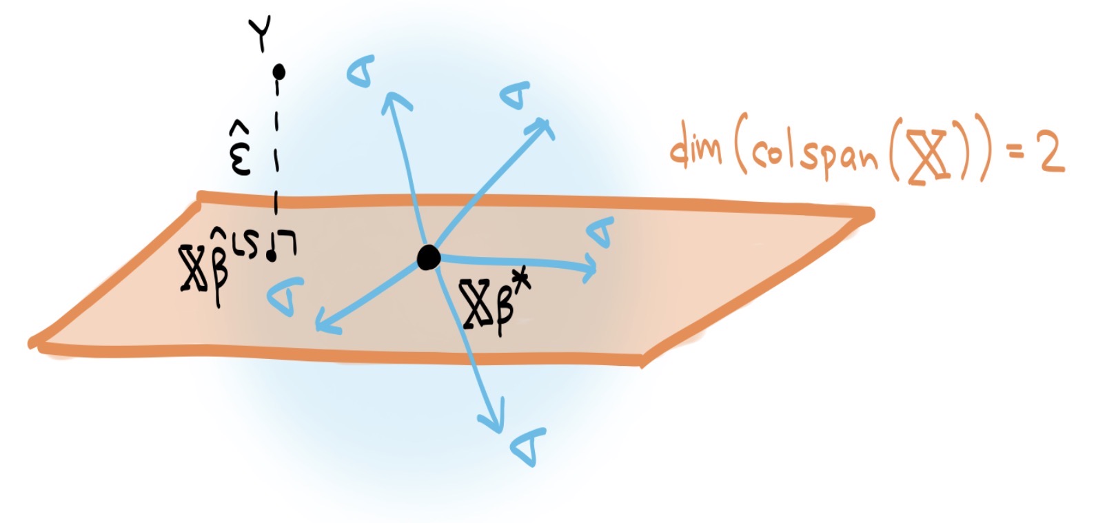
The above is an image outlining the ideas of the proof for $n = 5$ and $k = 2$ .

The orange subspace is the column span of $\mathbb{X}$ , with vector $\mathbb{X}\beta^*$ lying on it.
- We assume this subspace has dimension $k = 2$ .
The vector $Y$ is the result of taking $\mathbb{X}\beta^*$ and adding $5$ -dimensional Gaussian noise $\epsilon \sim \mathcal{N}_5(0, \sigma^2 I_5)$ .
The foot of the altitude of $Y$ onto the orange plane is $\mathbb{X}\hat{\beta}^{\mathrm{LS}}$ , and $\hat{\epsilon}$ is the altitude vector itself.
Crucially, only $3$ of the $5$ “directions” of Gaussian noise point orthogonally to the orange $2$ -dimensional subspace.
- It is only these $3$ directions of noise that contribute to the squared length of $\hat{\epsilon}$ .
- Thus, we might expect the squared length of $\hat{\epsilon}$ to be the sum of $3$ copies of $\sigma^2$ .

That's why we might expect $\mathbb{E}\left[\|\hat{\epsilon}\|^2\right] = 3\sigma^2$ ; in general, the coefficient of $3$ would be $n - k$ . The technical complexity of the proof comes from having to formalize the notion of “directions of noise”.

Proof: The first step is to rewrite $\hat{\epsilon}$ as the “orthogonal component” of the overall Gaussian noise $\epsilon$ .

Lemma 1. Let $H$ denote the $\mathbb{R}^n \to \mathbb{R}^n$ map given by projecting vectors onto the column space of $\mathbb{X}$ . Then $\hat{\epsilon} = (I_n - H)\epsilon$ .

Proof: Recalling from Lecture 23 that $HY = \mathbb{X}\hat{\beta}^{\mathrm{LS}}$ , we can rewrite the definition of $\hat{\epsilon}$ like so:
$\begin{align*}\hat{\epsilon} = Y - \mathbb{X}\hat{\beta}^{\mathrm{LS}} & = (I_n - H)Y \\ & = (I_n - H)(\mathbb{X}\beta^* + \epsilon) \\ & = (I_n - H)(\mathbb{X}\beta^*) + (I_n - H)\epsilon.\end{align*}$
However, $(I_n - H)(\mathbb{X}\beta^*) = 0$ because $\mathbb{X}\beta^*$ already lies on the column space of $\mathbb{X}$ —that is, because $H(\mathbb{X}\beta^*) = \mathbb{X}\beta^*$ . Then all that remains is the $\hat{\epsilon} = (I_n - H)\epsilon$ term, as promised. $\square$

Define the matrix $M := I_n - H$ ; think of $M$ not as a projection map, but as an “altitude” map. Then we seek to show that $\mathbb{E}\left[\left\|M\epsilon\right\|^2\right] = (n - k) \sigma^2$ , where $\epsilon \sim \mathcal{N}_n(0, \sigma^2 I_n)$ .

To proceed, we'll need some deeper linear algebra tricks; refer to 18.701 Notes for reference.

Lemma 2. The matrix $M$ diagonalizes as $M = U\Lambda U^{\top}$ , where:

The matrix $U$ is orthogonal.
The matrix $\Lambda$ is diagonal with $k$ zeroes and $n - k$ ones.

Proof: Note that $M$ is a real symmetric matrix, so the Spectral theorem applies. This, alone, already guarantees us that $M$ is expressible in the form $M = U \Lambda U^{\top}$ with $U$ orthogonal and $\Lambda$ diagonal.

It remains to study $\Lambda$ , or equivalently, to study the spectrum of $M$ . Recall that for the $k$ -dimensional subspace $W := \mathrm{colspan}(\mathbb{X})$ of $\mathbb{R}^n$ , the map $M$ takes vectors in $\mathbb{R}^n$ to their “altitudes” onto $W$ . Therefore,

Every vector along $W$ has eigenvalue zero.
Every vector along $W^{\perp}$ (the $(n - k)$ -dimensional subspace of vectors orthogonal to $W$ ) has eigenvalue one.

This implies the spectrum of $M$ contains $k$ zeroes and $(n - k)$ ones, proving the lemma's promise about $\Lambda$ . $\square$

Denote $\eta := U^{\top}\epsilon$ (that is, $\epsilon$ expressed in the eigenbasis of $M$ ). Using Lemma 2, we can rewrite $\|M\epsilon\|^2$ like so:

\| M\epsilon \|^2 = \| U\Lambda U^{\top} \epsilon \|^2 = \| \Lambda U^{\top} \epsilon \|^2 = \| \Lambda \eta \|^2 = \sum_{i = 1}^n \Lambda_{i, i}^2 \eta_i^2.

Note that the step $\|U\Lambda U^{\top}\epsilon\|^2 = \|\Lambda U^{\top}\epsilon\|^2$ comes from the orthogonality of $U$ ; rotating $\Lambda U^{\top}\epsilon$ via multiplication by $U$ does not change its magnitude. Now just one more lemma.

Lemma 3. We have $\mathbb{E}[\eta] = 0$ and $\Cov(\eta) = \sigma^2 I_n$ (the same moments as $\epsilon$ ). By corollary, $\mathbb{E}[\eta_i^2] = \sigma^2$ for all $i$ .

Proof: The point is that $U$ is orthogonal, so $U^{\top}U = I_n$ , making the covariance unchanged.
$\mathbb{E}[\eta] = U^{\top} \mathbb{E}[\epsilon] = 0 ~~~ \text{ and } ~~~ \Cov(\eta) = U^{\top}\Cov(\epsilon)U = \sigma^2 I_n \cdot U^{\top}U = \sigma^2 I_n. ~~~ \square$

By Lemma 3, taking expectations on both sides yields:

\mathbb{E}\left[ \|M\epsilon\|^2 \right] = \mathbb{E}\left[ \sum_{i = 1}^n \Lambda_{i, i}^2 \eta_i^2 \right] = \sum_{i = 1}^n \Lambda_{i, i}^2 \mathbb{E}\left[\eta_i^2\right] = \sum_{i = 1}^n \Lambda_{i, i}^2 \sigma^2.

Exactly $n - k$ terms have $\Lambda_{i, i} = 1$ , and the rest have $\Lambda_{i, i} = 0$ , so the summation evaluates to $(n - k) \sigma^2$ , as promised. $\blacksquare$

With all that out of the way… we can now construct confidence intervals and perform hypothesis tests with $\hat{\beta}^{\mathrm{LS}}$ .

Remark. Most of the time, these tests will ask for whether $\beta_i^* = 0$ or $\beta_i^* \neq 0$ for some particular entry $i$ of $\beta^*$ . This translates to asking whether the information communicated by the $i^{\text{th}}$ entry of a feature vector says anything about the response that the other entries do not already say.

§ Affine Linear Regression

Suppose I have a collection of data points $\{(X_i, Y_i)\}_{i = 1}^n$ on the coordinate plane, and I'd like to draw their line of best fit. In other words, I would like to find parameters $(\hat{\beta}_1^{\mathrm{LS}}, \hat{\beta}_0^{\mathrm{LS}})$ for which $Y_i \approx \hat{\beta}^{\mathrm{LS}}_1X_i + \hat{\beta}^{\mathrm{LS}}_0$ .

This is not the same as a one-dimensional linear regression, as that would only produce a model $Y_i \approx \hat{\beta}^{\mathrm{LS}}X_i$ . Fortunately, there's an easy adjustment we can make to linear regression to generalize it to affine models as well.

Idea. Pad every feature vector $X_i \in \mathbb{R}^k$ with an extra $1$ , extending it to $\mathbb{R}^{k + 1}$ . Then:

\underbrace{ \begin{pmatrix} Y_1 \\ Y_2 \\ \vdots \\ Y_n \end{pmatrix} }_{Y} \approx \underbrace{ \begin{pmatrix} 1 & \text{---} & X_1^{\top} & \text{---} \\ 1 & \text{---} & X_2^{\top} & \text{---} \\ \vdots & & \vdots & \\ 1 & \text{---} & X_n^{\top} & \text{---} \\ \end{pmatrix} }_{\mathbb{X}} \underbrace{ \begin{pmatrix} \beta_0 \\ \beta_1 \\ \vdots \\ \beta_k \end{pmatrix} }_{\hat{\beta}^{\mathrm{LS}}} = \begin{pmatrix} \text{---} & X_1^{\top} & \text{---} \\ & \vdots & \\ \text{---} & X_n^{\top} & \text{---} \\ \end{pmatrix} \begin{pmatrix} \beta_1 \\ \vdots \\ \beta_k \end{pmatrix} + \begin{pmatrix} \beta_0 \\ \vdots \\ \beta_0 \end{pmatrix}.

So drawing a line of best fit when the feature dimension is $k = 1$ is secretly a two-dimensional linear regression, where the first entry of $\hat{\beta}^{\mathrm{LS}}$ communicates the $y$ -intercept, and the second entry communicates the slope.

§ 1D Linear Regression and Correlation

Definition. Given one-dimensional data $X_1, \dots, X_n \in \mathbb{R}$ and $Y_1, \dots, Y_n \in \mathbb{R}$ , we may compute their sample variances and sample covariances like so:

S_{xx} := \frac{1}{n} \sum_{i = 1}^n (X_i - \bar{X}_n)^2 ~~~ \parallel ~~~ S_{yy} := \frac{1}{n} \sum_{i = 1}^n (Y_i - \bar{Y}_n)^2 ~~~ \parallel ~~~ S_{xy} := \frac{1}{n} \sum_{i = 1}^n (X_i - \bar{X}_n)(Y_i - \bar{Y}_n)

Definition. The correlation coefficient between the $\{X_i\}_{i = 1}^n$ and the $\{Y_i\}_{i = 1}^n$ is defined as $r := \frac{S_{xy}}{\sqrt{S_{xx}S_{yy}}}$ .

It turns out that in the case of one-dimensional line-of-best-fit (or 2D linear regression), we have the following:

Theorem. (1D Linear Regression Slope) In a one-dimensional line-of-best-fit $Y_i \approx \hat{\beta}^{\mathrm{LS}}_1X_i + \hat{\beta}^{\mathrm{LS}}_0$ , we have $\hat{\beta}^{\mathrm{LS}}_1 = \frac{S_{xy}}{S_{xx}}$ .

Proof: Details omitted; the proof is just unenlightening computation. $\blacksquare$

Now let $\hat{Y}_i := \hat{\beta}^{\mathrm{LS}}_1X_i + \hat{\beta}^{\mathrm{LS}}_0$ denote the value of $Y_i$ predicted by the line-of-best-fit (in contrast to the true value $Y_i$ ).

Theorem. (Correlation and Regression) We have that $\frac{\hat{Y}_i - \bar{Y}_n}{\sqrt{S_{yy}}} = r \cdot \frac{X_i - \bar{X}_n}{\sqrt{S_{xx}}}$ .

Proof: More computation; omitted. $\blacksquare$

And that's why AP Statistics makes you interpret the correlation coefficient by writing, “The constant $r^2$ represents the percent of the variation in the response that is explained by the linear relationship with the feature vector.”