MIT 6.790 — Lecture 14

Convolutional Neural Networks

§ Motivating Convolutional Neural Networks

Remark. These notes assume familiarity with convolutions, specifically for 2D images. See 6.300 for reference.

Suppose we want to build a neural network for classifying images. How many parameters would we need?

Problem. Suppose we take a $1000\,\mathrm{px} \times 1000\,\mathrm{px}$ image as the input to a neural network. If the first hidden layer has $1000$ features, then how many parameters connect the input layer to the first hidden layer?

Solution: The input layer has $10^6$ nodes, and the hidden layer has $10^3$ nodes, so the neural network between the input layer and the first hidden layer appears like a $K_{10^6, 10^3}$ graph. That's a total of $\boxed{10^9}$ parameters, one for each edge.

(And that's assuming the image is grayscale; adding color complicates things even more!)

That's too many to feasibly perform backpropagation on. The issue isn't the number of nodes in the layers—it's the number of parameters needed to describe the relationship between them.

Maybe we don't need the full $K_{10^6, 10^3}$ graph, though. Or maybe we don't need a unique parameter for every edge connecting an input node to the pre-activation of a node in the next layer.

Maybe there's a meaningful subfamily of linear maps on 2D images that requires far fewer parameters to specify…

§ Convolutions and Pooling

Technically, these 2D images aren't really 2D. Most images have color channels, too—three of them (RGB), to be precise. So more generally, we should think of each layer of our NN as being a three-dimensional $H \times W \times C$ grid of nodes.

The input layer might be a $1000 \times 1000 \times 3$ grid, for example. Importantly, our hidden layers might also have more than one channel. So our maps between layers must be able to meaningfully accept three-dimensional tensors as input.

We now introduce our two maps from 3D tensors to 3D tensors: pooling and convolving.

Definition. Given an $H \times W \times C$ image, we apply pooling to downsample the image down to $H' \times W' \times C$ .

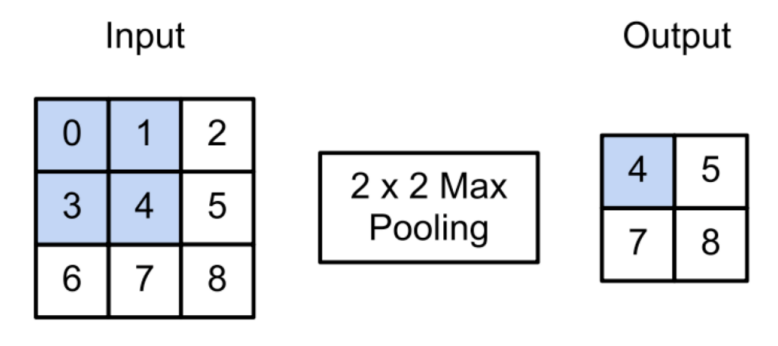
The image above depicts max pooling. There's also average pooling—you can probably imagine how that looks.

Remark. Pooling always treats each channel independently of every other. It may be more accurate to view pooling as a map from 2D tensors to smaller 2D tensors; to apply pooling on 3D tensors, simply apply pooling on each channel separately.

Definition. Given an $H \times W \times C$ image, we may convolve it using a $Y \times X \times C$ filter (with zero-padding). By sliding the filter along the width and height of the image, the resulting output is an $H \times W \times 1$ image.

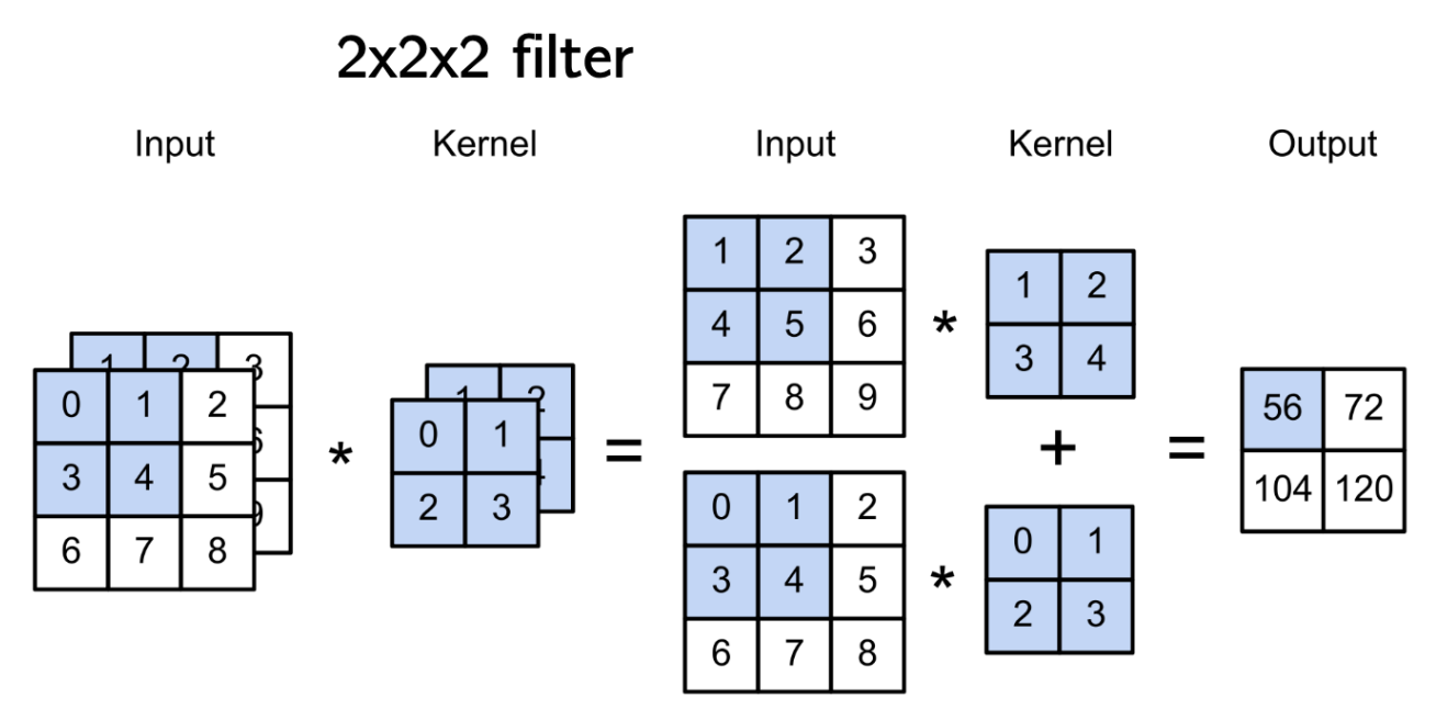
(The figure above omits zero-padding, so its output is smaller than its input.)

Remark. There are many possible variations of tensor convolution that one might imagine. For example, when sliding the filter, you might take a stride of length (say) $2$ . Then the output image instead has dimensions $\frac{H}{2} \times \frac{W}{2} \times 1$ .

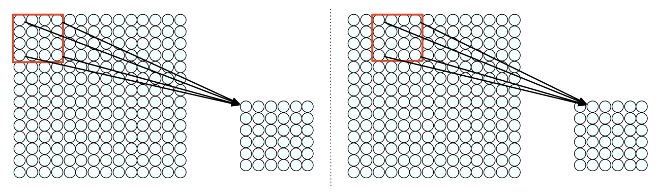
Ordinary convolution, by default, uses strides of length $1$ .

If we want the output of convolution to have more than one channel, we can simply stack convolutions together.

Definition. Given an $H \times W \times C$ image, we may perform stacked convolution using a $Y \times X \times C \times C'$ tensor of parameters. This tensor contains $C'$ different $Y \times X \times C$ filters stacked together. Applying each of the $C'$ filters to the input $H \times W \times C$ image yields $C'$ different $H \times W \times 1$ results. Stacking all $C'$ results together yields an $H \times W \times C'$ output image.

§ Convolutional Neural Networks

We can now put stacked convolution and pooling together to make a CNN. Here's an example.

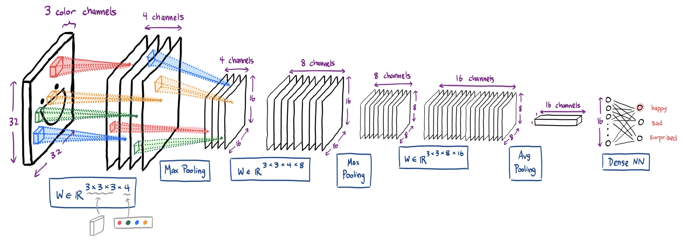
Let's walk through how this CNN works.

The input image is a $32 \times 32 \times 3$ image of a happy face.
To reach the $1^{\mathrm{st}}$ hidden layer, we apply a stacked convolution using a $3 \times 3 \times 3 \times 4$ tensor of parameters.
- The $1^{\mathrm{st}}$ hidden layer is then a $32 \times 32 \times 4$ image.
To reach the $2^{\mathrm{nd}}$ hidden layer, we apply max pooling to downsample the image to $16 \times 16 \times 4$ .
To reach the $3^{\mathrm{rd}}$ hidden layer, we apply a stacked convolution using a $3 \times 3 \times 4 \times 8$ tensor of parameters.
- The $3^{\mathrm{rd}}$ hidden layer is then a $16 \times 16 \times 8$ image.
To reach the $4^{\mathrm{th}}$ hidden layer, we apply max pooling to downsample the image to $8 \times 8 \times 8$ .
To reach the $5^{\mathrm{th}}$ hidden layer, we apply a stacked convolution using a $3 \times 3 \times 8 \times 16$ tensor of parameters.
- The $5^{\mathrm{th}}$ hidden layer is then an $8 \times 8 \times 16$ image.
To reach the $6^{\mathrm{th}}$ hidden layer, we apply average pooling to downsample the image to $1 \times 1 \times 16$ .
- The effect of average pooling here is to replace every $8 \times 8$ channel with the average of all $64$ of its pixel values.
Finally, we interpret the $6^{\mathrm{th}}$ hidden layer simply as $16$ nodes, and finish with an ordinary dense NN.
- Since the output layer has $3$ nodes, this is a $K_{16, 3}$ bipartite graph with $48$ edges (hence $48$ parameters).

And that's how a CNN works!

§ Commentary on CNNs

Some miscellaneous additional notes on CNNs:

Each stacked convolution only affects the number of channels, whereas each pooling only affects the width and height.
It was left unstated earlier, but after each convolution, a bias should be added to each cell, then a ReLU (or similar activation).
- Each channel gets a different bias that is added to every cell in that channel.
- So the $1^{\mathrm{st}}$ stacked convolution with a $3 \times 3 \times 3 \times 4$ tensor of parameters also requires $4$ bias parameters.
Compare the CNN above with an ordinary dense NN.
- In a dense NN, reaching the first layer would require $(32 \times 32 \times 3) \times (32 \times 32 \times 4)$ parameters.
- In this CNN, reaching the first layer only requires $3 \times 3 \times 3 \times 4 = 108$ parameters.
- Max pooling isn't implementable in an ordinary NN. And it requires zero parameters in this CNN.
- … something something, sparse matrices, something something …
Backpropagation is performed in the same way in CNNs as with NNs.
- The main difference is that each parameter now affects multiple pre-activations, not just one. But this just amounts to having to do more additions in the backwards pass.
In practice, here's what the learned filters for the first hidden layer might look like.

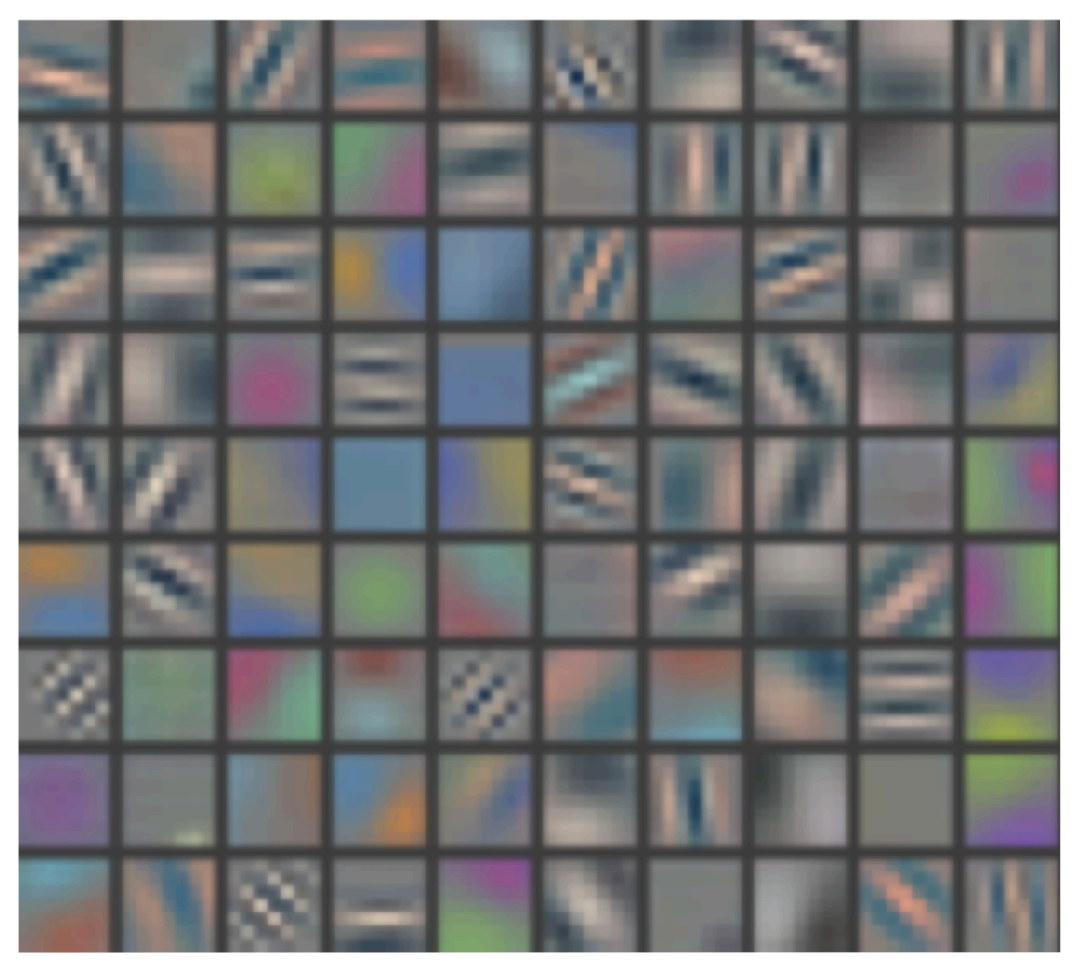
A lot of these filters should make sense from a signal processing perspective.

There are a lot more things that can be said about CNN architecture, including the endless possibilities for variations on the overall structure. Here's the structure of AlexNet—a highly-successful image classifier released in 2012—for example.

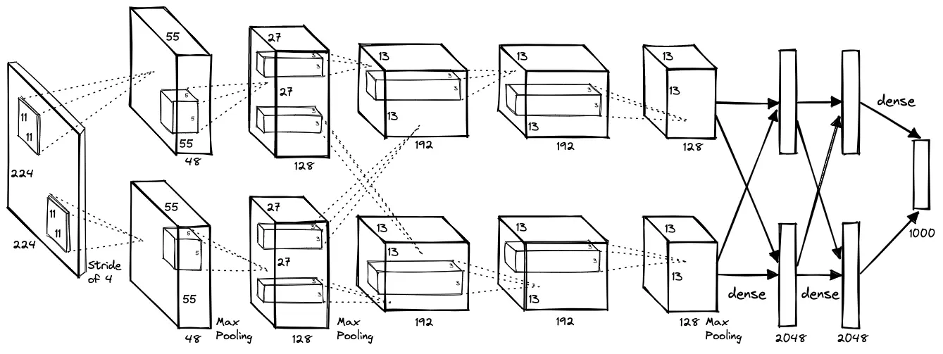
But we won't get into too much detail on that here.