MIT 6.300 — Lecture 17

2D Fourier Transform I

§ Lecture: 2D Fourier Series

For constructing 1D Fourier series, the main idea was that for a given period $T$ and fundamental frequency $\omega_0 = \frac{2\pi}{T}$ , the complex exponentials form an orthogonal basis.

\phi_{k}(t) := e^{jk \omega_0 t} \implies \left \langle \phi_{k_1}, \phi_{k_2} \right \rangle = \int_{T} \left[e^{-jk_1 \omega_0 t}\right] \cdot \left[e^{jk_2 \omega_0 t}\right] \, \mathrm{d}t = \begin{cases} T & \text{ if } k_1 = k_2 \\ 0 & \text{ otherwise.} \end{cases}

This generalizes readily to 2D Fourier series. We have a signal $f: \mathbb{R} \times \mathbb{R} \to \mathbb{C}$ with periods $T_x$ and $T_y$ along the $x$ and $y$ directions, with directional fundamental frequencies $\omega_{0, x} = \frac{2\pi}{T_x}$ and $\omega_{0, y} = \frac{2\pi}{T_y}$ . Then our orthogonal basis is:

\begin{align*}\phi_{k_x, k_y}(x, y) := e^{jk_x \omega_{0, x} x} \cdot e^{jk_y \omega_{0, y} y} ~ \implies ~~~~~~ & \left \langle \phi_{k_{x, 1}, k_{y, 1}}, \phi_{k_{x, 2}, k_{y, 2}} \right \rangle \\ = \ & \int_{T_x} \int_{T_y} \left[e^{-jk_{x, 1} \omega_{0, x} x} \cdot e^{-jk_{y, 1} \omega_{0, y} y}\right] \cdot \left[e^{jk_{x, 2} \omega_{0, x} x} \cdot e^{jk_{y, 2} \omega_{0, y} y}\right] \, \mathrm{d}y \, \mathrm{d}x \\ = \ & \begin{cases} T_x T_y & \text{ if } (k_{x, 1}, k_{y, 1}) = (k_{x, 2}, k_{y, 2}). \\ 0 & \text{ otherwise.} \end{cases}\end{align*}

By corollary, 2D Fourier series work like so:

Theorem. (2D CTFS) Given a periodic signal $f: \mathbb{R} \times \mathbb{R} \to \mathbb{C}$ , its Fourier series works like so.

F[k_x, k_y] := \frac{1}{T_xT_y} \int_{T_x} \int_{T_y} f(x, y) \left[e^{-jk_x \omega_{0, x} x} \cdot e^{-jk_y \omega_{0, y} y}\right] \, \mathrm{d}y \, \mathrm{d}x ~~~ \parallel ~~~ f(x, y) = \sum_{k_x = -\infty}^{\infty} \sum_{k_y = -\infty}^{\infty} F[k_x, k_y] \left[e^{jk_x \omega_{0, x} x} \cdot e^{jk_y \omega_{0, y} y}\right].

The 2D DTFS works exactly the same.

Theorem. (2D DTFS) Given a periodic signal $f: \mathbb{Z} \times \mathbb{Z} \to \mathbb{C}$ , its Fourier series works like so.

F[k_x, k_y] := \frac{1}{N_xN_y} \sum_{n_x = 0}^{N_x - 1} \sum_{n_y = 0}^{N_y - 1} f[n_x, n_y] \left[e^{-jk_x \Omega_{0, x} n_x} \cdot e^{-jk_y \Omega_{0, y} n_y}\right] ~~~ \parallel ~~~ f[n_x, n_y] = \sum_{k_x = 0}^{N_x - 1} \sum_{k_y = 0}^{N_y - 1} F[k_x, k_y] \left[e^{jk_x \Omega_{0, x} n_x} \cdot e^{jk_y \Omega_{0, y} n_y}\right].

§ Lecture: 2D Fourier Transform

Just as before, we care more about the CTFT and DTFT than we do the CTFS and DTFS. Their derivations work just as before.

Theorem. (2D CTFT) Given a signal $f: \mathbb{R} \times \mathbb{R} \to \mathbb{C}$ , its Fourier transform is:

F(\omega_x, \omega_y) := \int_{-\infty}^{\infty} \int_{-\infty}^{\infty} f(x, y) e^{-j(\omega_x x + \omega_y y)} \, \mathrm{d}x \, \mathrm{d}y ~~~ \parallel ~~~ f(x, y) = \frac{1}{4\pi^2} \int_{-\infty}^{\infty} \int_{-\infty}^{\infty} F(\omega_x, \omega_y) e^{j(\omega_x x + \omega_y y)} \, \mathrm{d}\omega_x \, \mathrm{d}\omega_y.

Proof: As in Lecture 6, take $f_{T_x, T_y}(x, y)$ to be the extension of $f(x, y)$ to have period $(T_x, T_y)$ . The CTFS of $f_{T_x, T_y}(x, y)$ is:

F_{T_x, T_y}[k_x, k_y] = \frac{1}{T_xT_y} \int_{T_x} \int_{T_y} f(x, y) \left[e^{-j\textcolor{#bf0140}{k_x \omega_{0, x}} x} \cdot e^{-j\textcolor{#bf0140}{k_y \omega_{0, y}} y}\right] \, \mathrm{d}y \, \mathrm{d}x

Now define the CTFT to be $F(\omega_x, \omega_y) := \lim_{(T_x, T_y) \to (\infty, \infty)} T_xT_y \cdot F_{T_x, T_y}[k_x, k_y]$ , where $\omega_x = k_x \omega_{0, x}$ and $\omega_y = k_y \omega_{0, y}$ are the reparametrization. First, check this matches the theorem statement.

F(\omega_x, \omega_y) = \lim_{(T_x, T_y) \to (\infty, \infty)} T_xT_y \cdot \left[ \frac{1}{T_xT_y} \int_{T_x} \int_{T_y} f(x, y) \left[e^{-j\textcolor{#bf0140}{k_x \omega_{0, x}} x} \cdot e^{-j\textcolor{#bf0140}{k_y \omega_{0, y}} y}\right] \, \mathrm{d}y \, \mathrm{d}x \right] = \int_{-\infty}^{\infty} \int_{-\infty}^{\infty} f(x, y) e^{-j(\textcolor{#bf0140}{\omega_x} x + \textcolor{#bf0140}{\omega_y} y)} \, \mathrm{d}x \, \mathrm{d}y.

Next, see what happens to the CTFS synthesis equation at the limit.

\begin{align*}f(x, y) & = \lim_{(T_x, T_y) \to (\infty, \infty)} \sum_{k_x = -\infty}^{\infty} \sum_{k_y = -\infty}^{\infty} F_{T_x, T_y}[k_x, k_y] \left[e^{j\textcolor{#bf0140}{k_x \omega_{0, x}} x} \cdot e^{j\textcolor{#bf0140}{k_y \omega_{0, y}} y}\right] \\ & = \lim_{(T_x, T_y) \to (\infty, \infty)} \sum_{k_x = -\infty}^{\infty} \sum_{k_y = -\infty}^{\infty} \textcolor{red}{\left[T_xT_y \cdot F_{T_x, T_y}[k_x, k_y]\right]} \left[e^{j\textcolor{#bf0140}{\omega_{k_x}} x} \cdot e^{j\textcolor{#bf0140}{\omega_{k_y}} y}\right] \left[\frac{1}{4\pi^2} \cdot \textcolor{red}{\frac{2\pi}{T_x}} \cdot \textcolor{red}{\frac{2\pi}{T_y}}\right] \\ & = \lim_{(T_x, T_y) \to (\infty, \infty)} \sum_{k_x = -\infty}^{\infty} \sum_{k_y = -\infty}^{\infty} \textcolor{red}{F(\omega_{k_x}, \omega_{k_y})} \left[e^{j\textcolor{#bf0140}{\omega_{k_x}} x} \cdot e^{j\textcolor{#bf0140}{\omega_{k_y}} y}\right] \left[\frac{1}{4\pi^2} \cdot \textcolor{red}{\Delta \omega_{k_x}} \cdot \textcolor{red}{\Delta \omega_{k_y}}\right] \\ & = \frac{1}{4\pi^2} \int_{-\infty}^{\infty} \int_{-\infty}^{\infty} F(\omega_x, \omega_y) e^{j(\omega_x x + \omega_y y)} \, \mathrm{d}\omega_x \, \mathrm{d}\omega_y.\end{align*}

To clarify: in the above, $\{\omega_{k_x}\}_{k_x = -\infty}^{\infty}$ denotes an arithmetic progression with common difference $\Delta \omega_{k_x} = \omega_{0, x} = \frac{2\pi}{T_x}$ . $\blacksquare$

Analogously, you can take the 2D DTFT as well.

Theorem. (2D DTFT) Given a signal $f: \mathbb{Z} \times \mathbb{Z} \to \mathbb{C}$ , its Fourier transform is:

F(\Omega_x, \Omega_y) := \sum_{n_x = -\infty}^{\infty} \sum_{n_y = -\infty}^{\infty} f[n_x, n_y] e^{-j(\Omega_x n_x + \Omega_y n_y)} ~~~ \parallel ~~~ f[n_x, n_y] = \frac{1}{4\pi^2} \int_{0}^{2\pi} \int_{0}^{2\pi} F(\Omega_x, \Omega_y) e^{j(\Omega_x n_x + \Omega_y n_y)} \, \mathrm{d}\Omega_x \, \mathrm{d}\Omega_y.

And of course, there's a 2D DFT as well, and it works just as before.

Theorem. (2D DFT) Given a DT signal $f[n_x, n_y]$ of size $N_x \times N_y$ , its discrete Fourier transform is:

F[k_x, k_y] := \frac{1}{N_xN_y} \sum_{n_x = 0}^{N_x - 1} \sum_{n_y = 0}^{N_y - 1} f[n_x, n_y] \left[e^{-jk_x \Omega_{0, x} n_x} \cdot e^{-jk_y \Omega_{0, y} n_y}\right] ~~~ \parallel ~~~ f[n_x, n_y] = \sum_{k_x = 0}^{N_x - 1} \sum_{k_y = 0}^{N_y - 1} F[k_x, k_y] \left[e^{jk_x \Omega_{0, x} n_x} \cdot e^{jk_y \Omega_{0, y} n_y}\right].

Remark. The 2D DFT is, up to a factor of $\frac{1}{N_xN_y}$ , the evaluation of the polynomial $p(z_x, z_y) := \sum_{n_x = 0}^{N_x - 1} \sum_{n_y = 0}^{N_y - 1} f[n_x, n_y] z_x^{n_x} z_y^{n_y}$ as $z_x$ and $z_y$ span the $N_x^{\text{th}}$ and $N_y^{\text{th}}$ roots of unity, respectively. And naturally, 2D circular convolution is just multivariate polynomial multiplication in the ring $\mathbb{C}[z_x, z_y]/(z_x^{N_x} - 1, z_y^{N_y} - 1)$ , and so on…

§ Recitation and Lecture: 2D DFT Algebraic Properties

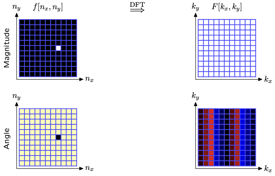
Theorem. (2D Unit-Sample DFT) The DFT of $f[n_x, n_y] := \delta[n_x] \delta[n_y]$ is the constant function $F[k_x, k_y] = \frac{1}{N_xN_y}$ .

Proof: Compare with the 1D case discussed in Lecture 7. Proof by plain computation. $\blacksquare$

Here's a useful trick for handling higher-dimension DFTs.

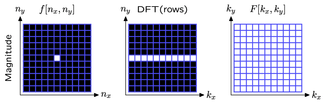
Theorem. (2D DFT Independence) To compute the size- $(N_x, N_y)$ DFT of $f[n_x, n_y]$ , it is equivalent to do the following.

First, replace every row with the size- $N_x$ DFT of that row.
Afterwards, replace every column with the size- $N_y$ DFT of that column.

Proof: Move the terms around between the double-summation.

F[k_x, k_y] = \overbrace{\frac{1}{N_y} \sum_{n_y = 0}^{N_y - 1} \underbrace{\left( \frac{1}{N_x} \sum_{n_x = 0}^{N_x - 1} f[n_x, n_y] e^{-jk_x\Omega_{0, x}n_x} \right)}_{ \text{row-wise DFT} } e^{-jk_y\Omega_{0, y} n_y}}^{\text{column-wise DFT}}.

Alternatively, adopt the polynomial interpretation: a multivariate polynomial in $(z_x, z_y)$ is just a single-variable polynomial in $z_y$ , where the coefficients are themselves polynomials in $z_x$ . $\blacksquare$

Here's a visual of how the trick above can be used to calculate the DFT of $f[n_x, n_y] = \delta[n_x]\delta[n_y]$ .

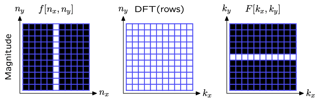
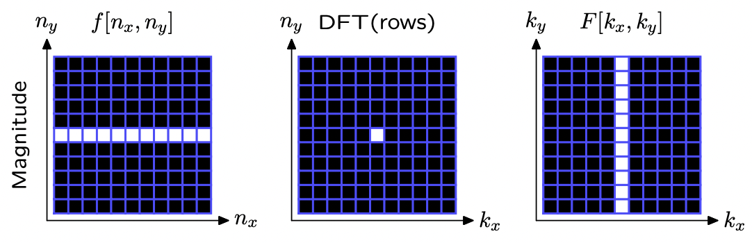
You can check for yourself the following facts, too:

The DFT of the constant signal $f[n_x, n_y] := 1$ is $F[k_x, k_y] = \delta[k_x]\delta[k_y]$ .
The DFT of the vertical-line signal $f[n_x, n_y] := \delta[n_x]$ is $F[k_x, k_y] = \frac{1}{N_x} \delta[k_y]$ (a horizontal line).
The DFT of the horizontal-line signal $f[n_x, n_y] := \delta[n_y]$ is $F[k_x, k_y] = \frac{1}{N_y} \delta[k_x]$ (a vertical line).
The DFT of an impulse train is another, perpendicular impulse train.

Here's one more trick: translation affects DFTs via phase shift. (Again, recall “Time Delay” from Lecture 7.)

Theorem. (2D DFT Translation) Given that $\mathrm{DFT}(f[n_x, n_y]) = F[k_x, k_y]$ , we have:

f'[n_x, n_y] := f[n_x - n_{x, 0}, n_y - n_{y, 0}] ~ \implies ~ \mathrm{DFT}(f'[n_x, n_y]) = e^{-jk_x\Omega_{0, x}n_{x, 0}} \cdot e^{-jk_y\Omega_{0, y}n_{y, 0}} F[k_x, k_y].

See below for the DFT of a translation of a unit-sample signal. Only the phase changes.

§ Lecture: 2D DFT Visual Properties

The key idea to keep in mind is the following:

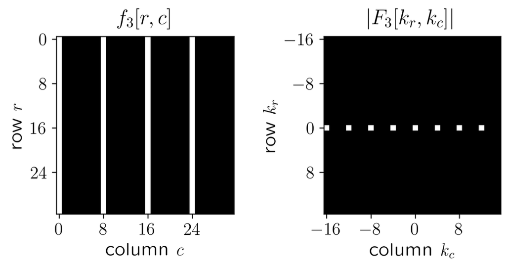
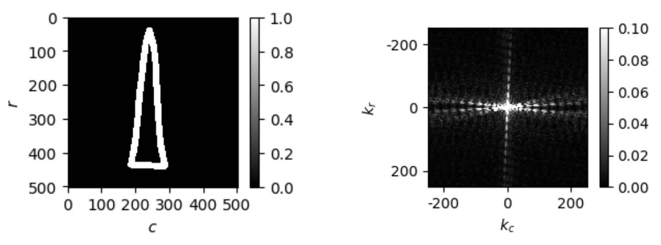
Idea. Lines in the space domain manifest as perpendicular lines in the frequency domain.

Here's an example of the DFT of a triangle. Notice how the DFT has three linear features, each perpendicular to a side of the triangle in the original signal.

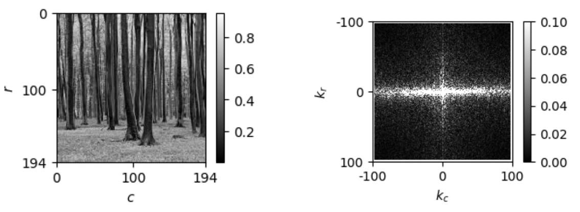
This photo of trees has strong vertical-line features, so its DFT has a strong horizontal line.

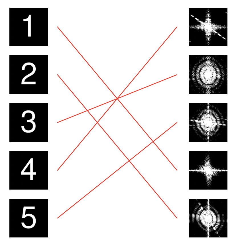
These are the DFTs of some digits.

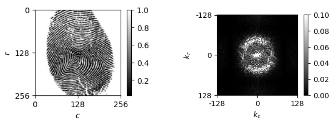
Here's an interesting one: the DFT of a fingerprint gives this bright ring of radius $\approx 40$ around a bright dot at the center.

The reason why is that a fingerprint locally is just a collection of evenly-spaced parallel lines. And a collection of evenly-spaced parallel lines is exactly what a 2D cosine wave looks like.

But the DFT of a 2D cosine wave is two dots, antipodal to one another on a circle of radius equal to the frequency of the cosine wave. Since a fingerprint consists of evenly-spaced parallel lines in all directions, those pairs of dots get rotated around this circle in all directions, forming the bright ring of radius $\approx 40$ .

In fact, a common preprocessing step in fingerprint analysis is to bandpass-filter around the ridge frequency—often implemented by keeping only that ring in the DFT before taking the inverse transform, yielding a high-contrast image of the ridges.