MIT 18.650 — Lecture 25

Logistic Regression

We now switch from linear regression to logistic regression. The only difference is that the response variable $Y$ now takes on a binary value: $Y \in \{0, 1\}$ .

Definition. Given data $\{(X_i, Y_i)\}_{i = 1}^n$ , with $X_i \in \mathbb{R}^k$ and $Y_i \in \{0, 1\}$ , our logistic regression model will be:

[Y \mid X = x] \sim \mathrm{Ber}\left( \sigma(x^{\top}\beta^*) \right) ~~~ \text{ where } ~~~ \sigma(t) := \frac{e^t}{1 + e^t}.

Note that $\sigma(t)$ is the sigmoid function, pictured below.

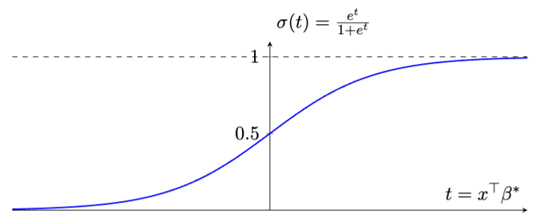
Note that the output $\sigma(x^{\top}\beta^*)$ of our regression model is not an estimate of the response, but rather an estimate of the probability that the response is equal to $1$ .

Remark. Another commonly-used model is the probit regression model, described below:

[Y \mid X = x] \sim \mathrm{Ber}\left( \Phi\left(x^{\top}\beta^*\right) \right) ~~~ \text{ where } ~~~ \Phi(t) \text{ is the CDF of } \mathcal{N}(0, 1).

An equivalent representation of the above model is:

Y = \mathds{1}(X^{\top}\beta^* + Z > 0) ~~~ \text{ where } ~~~ Z \sim \mathcal{N}(0, 1).

Not much is special about $\mathcal{N}(0, 1)$ , either. Any function $F(t)$ can replace the sigmoid function $\sigma(t)$ , so long as:

F(t) \text{ is increasing.} ~~~ \parallel ~~~ \lim_{t \to -\infty} F(t) = 0 \text{ and } \lim_{t \to \infty} F(t) = 1. ~~~ \parallel ~~~ F(0) = \frac{1}{2}.

§ MLE for Logistic Regression

Unfortunately, there is no closed-form expression for the MLE $\hat{\beta}^{\mathrm{MLE}}$ of logistic regression. But we can still do our best to try to approximate the log-likelihood-maximizer using gradient ascent.

Theorem. (Logistic Likelihood) The log-likelihood function for logistic regression is:

\ell_n(\beta) = \sum_{i = 1}^n \left[ Y_iX_i^{\top}\beta - \log\left( 1 + e^{X_i^{\top}\beta} \right) \right].

Proof: Recalling that $Y_i \mid X_i \sim \mathrm{Ber}\left( \sigma\left(X_i^{\top}\beta\right) \right)$ , the log likelihood is just

\begin{align*}\ell_n(\beta) & = \sum_{i = 1}^n \log\left( \sigma(X_i^{\top}\beta)^{Y_i} \cdot \left(1 - \sigma(X_i^{\top}\beta)\right)^{1 - Y_i} \right) \\ & = \sum_{i = 1}^n \left[ Y_i \log\left( \frac{\sigma(X_i^{\top}\beta)}{1 - \sigma(X_i^{\top}\beta)} \right) + \log(1 - \sigma(X_i^{\top}\beta)) \right] \\ & = \sum_{i = 1}^n \left[ Y_iX_i^{\top}\beta - \log\left( 1 + e^{X_i^{\top}\beta} \right) \right] ~~~ \text{ using the identities } \frac{\sigma(t)}{1 - \sigma(t)} = e^t \text{ and } 1 - \sigma(t) = \frac{1}{1 + e^t}.\end{align*}

And that's the furthest simplification can take us. $\blacksquare$

The upside is that the log likelihood is concave (proof omitted), so plain gradient ascent should work.

§ Multiclass Classification

A natural generalization of a binary response $Y \in \{0, 1\}$ is a multiclass response $Y \in \{0, 1, \dots, M\}$ .

The result of a multiclass logistic regression is a collection of $M$ parameters $(\beta_1^*, \beta_2^*, \dots, \beta_M^*)$ . These $M$ parameters collectively decide the behavior of $M + 1$ probability functions $(p_0(x), p_1(x), \dots, p_M(x))$ , where $\mathbb{P}[Y = m \mid X = x] = p_m(x)$ .

Remark. Check that this description is consistent with binary-classification logistic regression when $M = 1$ .

Also note that there are $M$ parameters, yet $M + 1$ probability functions; this is because the probability functions are constrained by the requirement that $\sum_{m = 0}^M p_m(x) = 1$ for all $x$ .

So how exactly do the parameters $\{\beta_m^*\}_{m = 1}^M$ relate to the probabilities $\{p_m(x)\}_{m = 0}^M$ in multiclass logistic regression?

Definition. Given data $\{(X_i, Y_i)\}_{i = 1}^n$ , with $X_i \in \mathbb{R}^k$ and $Y_i \in \{0, 1, \dots, M\}$ , our multiclass logistic regression model will be:

\mathbb{P}[Y = m \mid X = x] = p_m(x) ~~~ \parallel ~~~ p_0(x) = \frac{1}{1 + \sum_{j = 1}^M e^{x^{\top}\beta_j^*}} ~~~ \text{ and } ~~~ p_m(x) = \frac{e^{x^{\top}\beta_m^*}}{ 1 + \sum_{j = 1}^M e^{x^{\top}\beta_j^*} } ~ \text{ for all } m \neq 0.

Remark. It turns out that the log likelihood in multiclass logistic regression is the negative of the cross entropy loss from machine learning. (18.650 does not elaborate on this any further.)