MIT 18.650 — Lecture 23

Linear Regression I

Definition. In regression, our goal is to develop a model that, given a feature vector or predictor $X \in \mathbb{R}^k$ , outputs an estimate for a response variable $Y \in \mathbb{R}$ . The model's behavior is to be calibrated according to a training set $\{(X_i, Y_i)\}_{i = 1}^n$ .

Remark. Regression is like those puzzles that ask, “Given that $f(78) = 2$ , $f(89) = 3$ , and $f(90) = 2$ , what does $f(100)$ equal?” In this case, the training set is $\{(78, 2), (89, 3), (90, 2)\}$ , and we seek the response variable $Y$ to the feature vector $X = 100$ .

The scope of possible models is way too large; we need to make some assumptions about the relationship between $X$ and $Y$ .

§ Linear Regression MLE

Linear regression is driven by the following assumption.

Assumption. The distribution of $[Y \mid X = x]$ is $\mathcal{N}(f^*(x), \sigma^2)$ .

The standard deviation $\sigma$ is the same constant for all values of $x$ .
The mean function $f^*(x)$ is linear; that is, $f^*(x) = x^{\top}\beta^*$ for some $\beta^* \in \mathbb{R}^k$ .

Our regression model will thus also be a linear function $f(x) = x^{\top}\beta$ . So the goal of linear regression will be to construct a good point estimate $\beta$ of the true parameter $\beta^*$ .

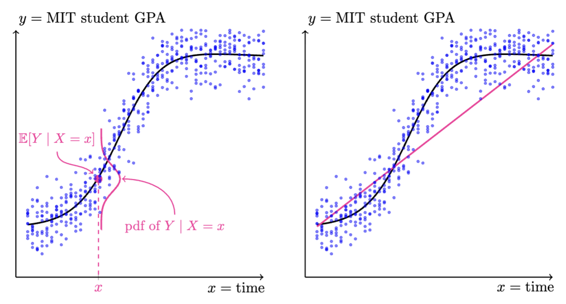
Remark. When we assume that the standard deviation is constant for all values of $x$ , we are using homoscedastic regression, as opposed to heteroscedastic regression.

We have a model $\{\mathbb{P}_{\beta} \mid \beta \in \mathbb{R}^k\}$ —that is, a collection of PDFs $\mathbb{P}_{\beta}$ , each on the space $\{(X, Y) \mid X \in \mathbb{R}^k, Y \in \mathbb{R}\}$ . We should pick the PDF $\mathbb{P}_{\beta}$ that makes the training data $\{(X_i, Y_i)\}_{i = 1}^n$ look as likely to have occurred as possible.

In other words, given the data $\{(X_i, Y_i)\}_{i = 1}^n$ , we'll just make our point estimate $\beta$ the MLE. (Recall Lecture 9.)

Theorem. (MLE = LS) The MLE $\hat{\beta}^{\mathrm{MLE}}$ minimizes squared-error training loss; that is,

\hat{\beta}^{\mathrm{MLE}} = \argmin_{\beta} \sum_{i = 1}^n (Y_i - X_i^{\top}\beta)^2.

Proof: The log likelihood $\ell_n(\beta)$ is:

\ell_n(\beta) = \sum_{i = 1}^n \log\left( \frac{1}{\sigma\sqrt{2\pi}} \exp\left[ -\frac{(Y_i - X_i^{\top}\beta)^2}{2\sigma^2} \right] \right) = -\frac{1}{2\sigma^2}\left[ \sum_{i = 1}^n (Y_i - X_i^{\top}\beta)^2 \right] + \text{constants}.

To maximize the log likelihood, we minimize the bracketed expression on the RHS, which is the squared-error training loss. $\blacksquare$

Remark. Suppose we instead said the distribution of $[Y \mid X = x]$ was $\mathcal{N}(f^*(x), \sigma(x)^2)$ —that is, suppose we performed heteroscedastic regression and did not assume the standard deviation was constant.

Then the MLE becomes the parameter that minimizes the sum of squares of z-scores; check for yourself. Note, however, that this MLE is not practical to compute, as the training data tells us nothing about z-scores because we do not know $\sigma(x)$ .

This is the reason why squared error is such a common loss function for regression: it's a natural consequence of seeking out the MLE assuming a Gaussian model.

§ Least Squares Loss

Definition. All training data is to be summarized in an $n \times 1$ column vector $Y$ and an $n \times k$ matrix $\mathbb{X}$ .

Y = \begin{pmatrix} Y_1 \\ Y_2 \\ \vdots \\ Y_n \end{pmatrix} \in \mathbb{R}^n ~~~ \text{ and } ~~~ \mathbb{X} = \begin{pmatrix} \text{---} & X_1^{\top} & \text{---} \\ \text{---} & X_2^{\top} & \text{---} \\ & \vdots & \\ \text{---} & X_n^{\top} & \text{---} \\ \end{pmatrix} \in \mathbb{R}^{n \times k}

Then the squared error rewrites as $\|Y - \mathbb{X}\beta\|^2$ , where $\beta \in \mathbb{R}^k$ .

Theorem. (Least Squares Solution) The LS (least squares) solution (also the MLE) is $\hat{\beta} = (\mathbb{X}^{\top}\mathbb{X})^{-1}\mathbb{X}^{\top}Y$ .

Proof: The gradient of the squared error $L(\beta) := \|Y - \mathbb{X}\beta\|^2$ is:

\nabla_{\beta} L(\beta) = -2\mathbb{X}^{\top}(Y - \mathbb{X}\beta) = 2 \left[ \mathbb{X}^{\top}\mathbb{X}\beta - \mathbb{X}^{\top}Y \right].

Setting this equal to zero yields the promised result. $\blacksquare$

Remark. When setting $\nabla_{\beta}L(\beta)$ to zero, we can't just set $Y - \mathbb{X}\beta$ to zero, because $\mathbb{X}^{\top}$ isn't necessarily invertible.

Note, furthermore, that $\hat{\beta} = (\mathbb{X}^{\top}\mathbb{X})^{-1}\mathbb{X}^{\top}Y$ may not be well-defined, as $\mathbb{X}^{\top}\mathbb{X}$ may not be invertible. As the next section may make more clear, it is possible that there are multiple LS solutions, all equally valid according to the limited training data provided.

However, at least one candidate for $\hat{\beta}$ always exists; the minimum loss has to be achieved by something.

And so $\beta$ is the $k$ -dimensional vector that holds the coefficients to our linear regression $f \colon \mathbb{R}^k \to \mathbb{R}$ via $f(x) := x^{\top}\beta$ .

§ Interpreting the LS Solution

We now do some linear algebra to interpret the vector $\beta = (\mathbb{X}^{\top}\mathbb{X})^{-1}\mathbb{X}^{\top}Y \in \mathbb{R}^k$ .

Theorem. (LS = Projection Coefficients) The vector $\mathbb{X}\beta \in \mathbb{R}^n$ is the projection of $Y \in \mathbb{R}^n$ onto the column space of $\mathbb{X}$ .

Proof: It's clear that $\mathbb{X}\beta$ lives in the column space of $\mathbb{X}$ ; it is true for any vector $\beta \in \mathbb{R}^k$ that:

\mathbb{X}\beta = \beta_1 \mathrm{col}_1(\mathbb{X}) + \beta_2 \mathrm{col}_2(\mathbb{X}) + \dots + \beta_k \mathrm{col}_k(\mathbb{X}).

It remains to verify that $Y - \mathbb{X}\beta$ is perpendicular to this column space; algebraically, that $\mathbb{X}^{\top}(Y - \mathbb{X}\beta) = 0$ . And, well, the proof of this lives within the very derivation of $\beta$ itself, right in the body of the “Least Squares Solution” proof. $\blacksquare$

An equivalent statement of the above is that the linear regression $f \colon \mathbb{R}^k \to \mathbb{R}$ via $f(x) := x^{\top}\beta$ is such that:

\mathbb{X}\beta = \begin{pmatrix} f(X_1) \\ f(X_2) \\ \vdots \\ f(X_n) \end{pmatrix} \text{ is as close to } Y = \begin{pmatrix} Y_1 \\ Y_2 \\ \vdots \\ Y_n \end{pmatrix} \text{ as possible.}

Indeed, $\mathbb{X}\beta$ must live in the column space of $\mathbb{X}$ , and the closest point from $Y$ to this column space is the projection.

And really, the above statement should have been predictable from the very beginning. The squared distance between $\mathbb{X}\beta$ and $Y$ is exactly the squared-error training loss, so minimizing this loss is equivalent to making $\mathbb{X}\beta$ and $Y$ as close as possible.

In that sense, the vector $\beta = (\mathbb{X}^{\top}\mathbb{X})^{-1}\mathbb{X}^{\top}Y \in \mathbb{R}^k$ is just symbolic notation for the coefficients of the weighted sum of the columns of $\mathbb{X}$ that lands as close to $Y$ as possible.