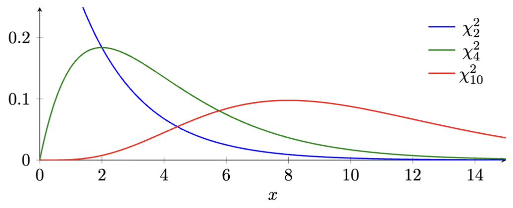
Definition. A random variable X is said to have “a χ2 distribution with k degrees of freedom”, denoted X∼χk2, if and only if X is distributed as Z12+⋯+Zk2, where {Zi}i=1k are i.i.d. samples from N(0,1).
Note that E[X]=k and V[X]=2k if X∼χk2.
Definition. The upper α quantile of the χk2 distribution is denoted χk,α2, where P(X>χk,α2)=α given X∼χk2.
§ Goodness of Fit Tests
Suppose we have a random variable X that takes on k discrete values {1,2,…,k}. For example, X might be the color of a randomly selected jellybean, either red, green, blue, or black.
Suppose such a random variable X has a true PMF f:{1,2,…,k}→[0,1] and an expected PMF f0. A goodness of fit test determines whether H0:f=f0 or H1:f=f0.
Theorem. (Pearson's χ2 GoF Test) Suppose we seek a goodness of fit test with level α as described above, and our data consists of n samples {Xi}i=1n taken (i.i.d.) from X.
Using the data, compute {O1,O2,…,Ok} where Oj is the # of the {Xi}i=1n that are equal to j.
Using the expected PMF f0, compute {E1,E2,…,Ek}, where Ej is the “expected” count Ej:=nf0(j) assuming H0.
Then our test statistic is Tn:=∑j=1kEj(Oj−Ej)2, we claim that under H0, we have Tn⇝χk−12 as n→∞, and our test is Ψ:=1(Tn>χk−1,α2).
Proof: The mathematically-nontrivial part of this test is the claim that Tn⇝χk−12 as n→∞. The proof of this claim is fairly computationally intensive, so we omit it here. (18.650 does not cover it.) ■
§ The T-Test
Recall that the Wald test for population means relies on the following two approximations:
The test statistic Tn:=σ/nXˉn−μ is approximately N(0,1) by the CLT.
We can approximate σ≈σ^:=sn2 by the LLN, CLT, and Slutsky's. (See Lectures 1-3 notes.)
Suppose that our population distribution is normal: X∼N(μ,σ2). Then approximation #1 holds—it's not even an approximation! But for small n, approximation #2, which says Tn≈σ^/nXˉn−μ, needs refinement.
Theorem. (T-Test) Suppose X1,…,Xn∼N(μ,σ2) (i.i.d.) and σ^2=n−11∑i=1n(Xi−Xˉn)2. Then we have:
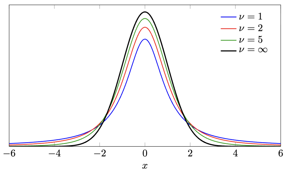
σ^/nXˉn−μ∼tn−1 where tν has PDF f(x):=νπ⋅Γ(2ν)Γ(2ν+1)(1+νx2)−(ν+1)/2.
We say that tν is the Student's t-distribution (named after the pseudonym “Student” used by William Sealy Gosset).
Again, we won't give the mathematical justification as it gets too involved.