MIT 18.650 — Lecture 19

Non-parametric Tests

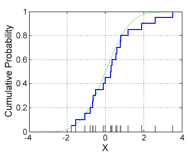
So far, we've only looked at tests for parameters of a distribution. Non-parametric tests refer to tests about the distribution as a whole; the three examples of such tests we'll discuss in this lecture are:

Kolmogorov-Smirnov. Given $X_1, \dots, X_n$ sampled (i.i.d.) from a distribution with CDF $F$ , we have:
$H_0 := \text{``The CDF $F$ matches another CDF $F_0$.''} ~~~ \parallel ~~~ H_1 := \text{``The CDF $F$ does not match another CDF $F_0$.''}$
Kolmogorov-Lilliefors. Given $X_1, \dots, X_n$ sampled (i.i.d.) from a distribution $X \sim \mathbb{P}$ , we have:
$H_0 := \text{``The random variable $X$ is Gaussian.''} ~~~ \parallel ~~~ H_1 := \text{``The random variable $X$ is not Gaussian.''}$
Two-Sample Test. Given $X_1, \dots, X_n \sim F_X$ and $Y_1, \dots, Y_m \sim F_Y$ (i.i.d.), where $F_X$ and $F_Y$ are CDFs, we have:
$H_0 := \text{``The CDF $F_X$ matches the CDF $F_Y$.''} ~~~ \parallel ~~~ H_1 := \text{``The CDF $F_X$ does not match the CDF $F_Y$.''}$

All three of these tests share the same idea behind their test statistic.

Definition. Given $X_1, \dots, X_n$ sampled (i.i.d.) from a distribution, their empirical CDF is $\hat{F}_n(t) := \frac{1}{n} \sum_{i = 1}^n \mathds{1}(X_i \leq t)$ .

Then the test statistic for all three tests will look something like $T_n := \sup_t \left|\hat{F}_n(t) - F_0(t)\right|$ , which represents the greatest absolute difference between the empirical CDF $\hat{F}_n(t)$ and the expected CDF $F_0(t)$ .

§ The Kolmogorov-Smirnov Test

Here's the main idea behind the test.

Theorem. (Kolmogorov-Smirnov Distribution) Assuming the null hypothesis, suppose $X_1, \dots, X_n$ are sampled (i.i.d.) from the distribution with continuous CDF $F_0$ . Then the distribution of the test statistic $T_n$ does not depend on $F_0$ .

Remark. This should not be particularly surprising. For example, it should be clear why $F_0(t)$ and $F_0(\frac{t}{2})$ would yield the same test statistic: scaling the $x$ -axis of a CDF shouldn't affect the maximum-detected difference in $y$ -values.

Proof: The point is that the CDF $F_0$ has no relevance at all, and the lemma below explains why.

Lemma. If a random variable $X$ has continuous CDF $F_0$ , then $F_0(X) \sim \mathrm{Unif}(0, 1)$ .

Proof: Ignoring the real-analysis technicalities, here's the gist of why this should feel true.

When we say $X$ has continuous CDF $F_0$ , that just means $X$ can be generated by picking a random number $\lambda \sim \mathrm{Unif}(0, 1)$ , then setting $X = F_0^{-1}(\lambda)$ . The conclusion is immediate from here. $\square$

The above lemma lets us rewrite the empirical distribution, which then lets us write the test statistic $T_n$ with no reference to $F_0$ . Below, we set $U_i := F_0(X_i)$ , so that by the lemma, these are all i.i.d. samples from $\mathrm{Unif}(0, 1)$ .

\begin{align*}T_n = \sup_{t \in \mathbb{R}} \left|\hat{F}_n(t) - F_0(t)\right| & = \sup_{t \in \mathbb{R}} \left|\left[ \frac{1}{n}\sum_{i = 1}^n \mathds{1}(X_i \leq t) \right] - F_0(t)\right| \\ & = \sup_{t \in \mathbb{R}} \left|\left[ \frac{1}{n}\sum_{i = 1}^n \mathds{1}(U_i \leq F_0(t)) \right] - F_0(t)\right| = \sup_{s \in [0, 1]} \left|\left[ \frac{1}{n}\sum_{i = 1}^n \mathds{1}(U_i \leq s) \right] - s\right| \sim \mathrm{KS}_n.\end{align*}

That last expression is the definition of the Kolmogorov-Smirnov distribution $\mathrm{KS}_n$ , which does not depend on $F_0$ . $\blacksquare$

And, of course, the above theorem easily gives rise to a Kolmogorov-Smirnov Test of level $\alpha$ . Just compute the test statistic $T_n$ and reject $H_0$ if $T_n > \mathrm{KS}_{n, \alpha}$ .

§ The Kolmogorov-Lilliefors Test

To test whether a random variable is Gaussian, we rework our test statistic like so:

T_n := \sup_t\left| \hat{F}_n(t) - \Phi_{\hat{\mu}, \hat{\sigma}^2}(t) \right| ~~~ \text{ where } ~~~ \hat{\mu} = \text{sample mean} ~~~ \text{ and } ~~~ \hat{\sigma}^2 = \text{sample variance}

Theorem. (Kolmogorov-Lilliefors Distribution) Assuming the null hypothesis, suppose $X_1, \dots, X_n$ are sampled (i.i.d.) from the distribution $\mathcal{N}(\mu, \sigma^2)$ . Then the distribution of the test statistic $T_n$ does not depend on $\mu$ or $\sigma^2$ .

Remark. This one really shouldn't be unexpected. It should be clear why the CDFs $F_0(t)$ and $F_0\left(\frac{t - \mu}{\sigma}\right)$ would yield the same test statistic, because scaling or shifting the $x$ -axis shouldn't affect the maximum-detected difference in $y$ -values.

Proof: Say that $X_i = \mu + \sigma \cdot Z_i$ , where $Z_1, \dots, Z_n \sim \mathcal{N}(0, 1)$ . The goal is to rewrite $T_n$ so that its value is dependent only on the values of $\{Z_i\}_{i = 1}^n$ (which, of course, do not depend on $\mu$ or $\sigma^2$ ).

Here are the relevant lemmas. Their proofs are very straightforward.

Lemma 1. Let $\hat{G}_n(t)$ denote the empirical CDF of the $\{Z_i\}_{i = 1}^n$ . Then $\hat{F}_n(t) = \hat{G}_n\left( \left[\frac{t - \mu}{\sigma}\right] \right)$ .

Lemma 2. We have $\hat{\sigma}^2 = \sigma^2 \cdot \hat{\sigma}_{Z, n}^2$ , where $\hat{\sigma}_{Z, n}$ is a function of only the $\{Z_i\}_{i = 1}^n$ .

Lemma 3. As a corollary of Lemma 2, if $\Phi$ is the CDF of $\mathcal{N}(0, 1)$ , then we have:
$\Phi_{\hat{\mu}, \hat{\sigma}^2}(t) = \Phi\left(\frac{t - \bar{X}_n}{\hat{\sigma}}\right) = \Phi\left(\frac{ t - \mu - \sigma \cdot \bar{Z}_n }{ \sigma \cdot \hat{\sigma}_{Z, n} }\right) = \Phi\left( \frac{\left[\frac{t - \mu}{\sigma}\right] - \bar{Z}_n}{\hat{\sigma}_{Z, n}} \right).$

Using Lemma 1 and Lemma 3, we can now rewrite $T_n$ like so:

T_n = \sup_{t \in \mathbb{R}} \left| \hat{F}_n(t) - \Phi_{\hat{\mu}, \hat{\sigma}^2}(t) \right| = \sup_{t \in \mathbb{R}} \left| \hat{G}_n\left( \left[\frac{t - \mu}{\sigma}\right] \right) - \Phi\left( \frac{\left[\frac{t - \mu}{\sigma}\right] - \bar{Z}_n}{\hat{\sigma}_{Z, n}} \right) \right| = \sup_{s \in \mathbb{R}} \left| \hat{G}_n(s) - \Phi\left(\frac{s - \bar{Z}_n}{\hat{\sigma}_{Z, n}}\right) \right| \sim \mathrm{KL}_n.

The RHS of the above is dependent only on the $\{Z_i\}_{i = 1}^n$ , so its distribution is dependent only on $n$ . It follows the Kolmogorov-Lilliefors distribution $\mathrm{KL}_n$ . $\blacksquare$

And, of course, you get a Kolmogorov-Lilliefors test out of this, too.

Remark. It turns out that $\mathrm{KL}_{n, \alpha} < \mathrm{KS}_{n, \alpha}$ for all $n$ . This means that if we mistakenly used the $\mathrm{KS}$ quantiles for a KL test, we would reject the null too infrequently.

§ The Two-Sample Test

To check if two sets of samples $\{X_i\}_{i = 1}^n$ and $\{Y_i\}_{i = 1}^m$ came from the same CDF, we use the following test statistic:

T_{n, m} := \sup_t \left| \hat{F}_{X, n}(t) - \hat{F}_{Y, m}(t) \right|.

Theorem. (Two-Sample Distribution) Assuming the null hypothesis, suppose $\{X_i\}_{i = 1}^n$ and $\{Y_i\}_{i = 1}^m$ are both sampled from the same continuous CDF $F$ . Then the distribution of the test statistic $T_{n, m}$ does not depend on $F$ .

Proof: Same proof as with the $\mathrm{KS}$ distribution. Say $U_i := F(X_i)$ and $V_i := F(Y_i)$ , which by the lemma are i.i.d. samples from $\mathrm{Unif}(0, 1)$ . Then:

\begin{align*}T_{n, m} & = \sup_{t \in \mathbb{R}}\left| \left[\frac{1}{n}\sum_{i = 1}^n \mathds{1}(X_i \leq t)\right] - \left[\frac{1}{m}\sum_{i = 1}^m \mathds{1}(Y_i \leq t)\right] \right| \\ & = \sup_{t \in \mathbb{R}}\left| \left[\frac{1}{n}\sum_{i = 1}^n \mathds{1}(U_i \leq F(t))\right] - \left[\frac{1}{m}\sum_{i = 1}^m \mathds{1}(V_i \leq F(t))\right] \right| \\ & = \sup_{s \in [0, 1]}\left| \left[\frac{1}{n}\sum_{i = 1}^n \mathds{1}(U_i \leq s)\right] - \left[\frac{1}{m}\sum_{i = 1}^m \mathds{1}(V_i \leq s)\right] \right|.\end{align*}

And that doesn't depend on $F$ . $\blacksquare$

And, yeah, you can perform tests with this, too.