MIT 18.650 — Lecture 21
Bayesian Inference I
§ Review: Likelihood and Multivariate Distributions
Suppose we have independent random variables , each with a PDF with a dependency on a parameter . As an example, we might have something like .
If we're given the values , that lets us compute a likelihood function that tells us how likely it would be to have observed this data given that the parameter had value . (Recall Lecture 9.)
In the above, is the joint PDF. (Recall Lecture 6.)
§ Priors and Posteriors
Now suppose we have some prior belief about the distribution of the parameter . As an example, perhaps is a probability that we believe to be more likely to be high than low.
Definition. A prior is a PDF that describes the probability distribution taken on by the parameter .
We now read in some data that has a dependency on . Bayes' rule tells us the following:
The LHS is our updated, posterior belief about the distribution of the parameter .
Remark. Notice how we don't care about the exact value of , because it is effectively a normalizing constant that works only to make the integral of equal to one.
Definition. The posterior is the probability distribution proportional to .
§ Conjugate Priors
Definition. The Beta distribution (where ) has PDF given by .
Remark. For example, the PDF of is .
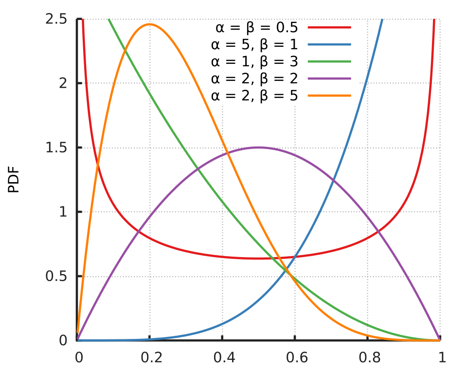
Example. Suppose we sample data i.i.d. from , and our prior is . In terms of the data , what is the posterior distribution?
Solution: Suppose of the samples are one, and the remaining samples are zero. Then we have:
Therefore, the posterior distribution is .
Definition. If the prior and posterior live in the same family of distributions, we say that we have a conjugate prior.
Remark. In the previous example, was a conjugate prior. But this fact relies on the distributions of the sample data all being , rather than, say, .
§ Bayes Estimator and Max A Posteriori
As we read in more data, our posterior distribution becomes more informative. In fact, one can show that the standard deviation of the posterior decreases as with the number of samples .
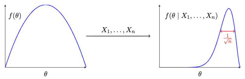
Eventually, we might want to summarize the posterior distribution with a single point estimate for .
Definition. The Bayes estimator (or mean a posteriori) is the expected value of under the posterior distribution.
Definition. The max a posteriori (MAP) is the mode of the posterior; that is, the value of that maximizes .
Generally, the MAP is much easier to compute than the Bayes estimator, because it doesn't require computing any normalizing factors.
Remark. If we have no priors at all—that is, our prior is the uniform distribution—then the max a posteriori is just the MLE. The spirit of Bayesian inference is that we must now account for priors.