MIT 18.650 — Lecture 20

Permutation Test and Multiple Hypothesis Testing

§ The Permutation Test

Just one more test to discuss. This one has the same hypotheses as the two-sample test from Lecture 19.

Permutation Test Hypotheses. Given $X_1, \dots, X_n \sim F_X$ and $Y_1, \dots, Y_m \sim F_Y$ (i.i.d.), where $F_X$ and $F_Y$ are CDFs, we have:
$H_0 := \text{``The CDF $F_X$ matches the CDF $F_Y$.''} ~~~ \parallel ~~~ H_1 := \text{``The CDF $F_X$ does not match the CDF $F_Y$.''}$

The test statistic for the permutation test is simply $T := |\bar{X}_n - \bar{Y}_m|$ . It remains to determine a threshold $t_{\alpha}$ for which, under the null hypothesis, the probability that $T > t_{\alpha}$ is below $\alpha$ .

Remark. Note that if $F_X$ and $F_Y$ are different distributions but have the same mean, we will likely commit a Type II error. The two-sample test is more robust than the permutation test in this regard.

Combine all $m + n$ samples into a single list $\{Z_i\}_{i = 1}^{m + n}$ , where the first $n$ samples are $\{X_i\}_{i = 1}^n$ and the last $m$ samples are $\{Y_i\}_{i = 1}^m$ . If the null hypothesis is true, then all permutations of $\{Z_i\}_{i = 1}^{m + n}$ are equally likely to occur from this process.

Thus, we can estimate the expected distribution of the test statistic $T$ under the null hypothesis by iterating over all permutations $\pi \colon [m + n] \to [m + n]$ , and for each permutation, compute its corresponding test statistic.

T_{\pi} = \left| \left[\frac{1}{n}\sum_{i = 1}^n Z_{\pi(i)}\right] - \left[\frac{1}{m}\sum_{i = 1}^m Z_{\pi(i + n)}\right] \right|.

Then just pick $t_{\alpha}$ to be the $(1 - \alpha)^{\text{th}}$ quantile across all $(m + n)!$ values of $T_{\pi}$ . That's it.

Remark. In practice, iterating through all $(m + n)!$ permutations $\pi$ is too computationally inefficient. So we usually just sample $M$ random permutations instead, then compute the quantile using this approximate data.

§ Multiple Hypothesis Testing

Here's the relevant xkcd for this section.

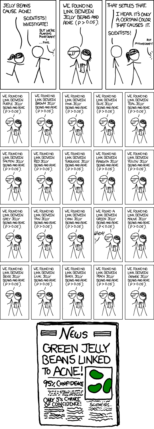
Type I errors (i.e. the null hypothesis is rejected even though it is true) accumulate when hypothesis testing is repeated multiple times. For example, if the null hypothesis is true, then a hypothesis test at level $\alpha = 0.05$ might have a $5\%$ chance of yielding a Type I error. Formally, here is the justification of why this is true.

Theorem. (P-Values Are Uniform) If the null hypothesis is true, then the p-value follows a uniform distribution.

Proof: Suppose that, under the null hypothesis, the test statistic $T$ has continuous (for simplicity) CDF $F$ . Also assume (WLOG) that we are performing a one-sided test where we reject if $T$ exceeds some quantile $c_{\alpha}$ .

The key is the following lemma stated earlier in Lecture 19.

Lemma. If $T \sim F$ , then $F(T) \sim \mathrm{Unif}(0, 1)$ . (And, assuming the null hypothesis, we do in fact have $T \sim F$ here.)

For this kind of test, the p-value is $p = 1 - F(T)$ . Thus, since $F(T)$ is uniform, so is $p$ . $\blacksquare$

§ The Bonferroni Correction

Here's one easy way to fix this: if you're performing $m$ tests, then you should divide the level $\alpha$ of your test by $m$ .

Definition. When performing $m$ tests, the family-wise error rate (FWER) is the probability of making at least one Type I error, assuming the null hypothesis is true in all cases.

Definition. When performing $m$ tests, we use the Bonferroni correction: reject the $i^{\text{th}}$ test if its p-value is at most $\alpha/m$ . Doing so will ensure the FWER is at most $\alpha$ , assuming the null hypothesis is true in all cases.

The proof why the Bonferroni correction works is just the union bound, followed by invoking the uniformity of p-values.

\mathbb{P}_{H_0}\left( \bigcup_{i = 1}^m \text{``}H_{0, i} \text{ is rejected}\text{''} \right) \leq \sum_{i = 1}^m \mathbb{P}_{H_0}\left( \text{``}H_{0, i} \text{ is rejected}\text{''} \right) = \sum_{i = 1}^m \mathbb{P}_{H_0}\left( p_i \leq \frac{\alpha}{m} \right) = \alpha.

There are some problems with the Bonferroni correction, though. For one, it's too tight. If $m = 1000$ , then $\alpha / m$ will be far too low to actually reject any tests.

Furthermore, the Bonferroni correction is calibrated for the worst case, where all null hypotheses are true. But if some null hypotheses are false, then we really should expect some positives, and we really ought to be more lenient.

Perhaps we should instead be working only, more weakly, to limit the proportion of positives that are false positives…

§ The Benjamini-Hochberg Method

Definition. The false discovery proportion (FDP) is $\text{FDP} := \frac{\# \text{ false positives}}{\# \text{ positives}}$ , taken to be $0$ when there are no positives.

Definition. The false discovery rate (FDR) is the expected value of the FDP.

Remark. If the null hypothesis is true in all cases, then all positives are false positives. In this case, we have:

\text{FDP} = \begin{cases} 1 & \text{ if at least one Type I error is made.} \\ 0 & \text{ if no Type I errors are made.} \end{cases}

Therefore, if the null hypothesis is true in all cases, the FDR equals the FWER.

Instead of aiming for $\text{FWER} \leq \alpha$ , the Benjamini-Hochberg (BH) method aims for $\text{FDR} \leq \alpha$ .

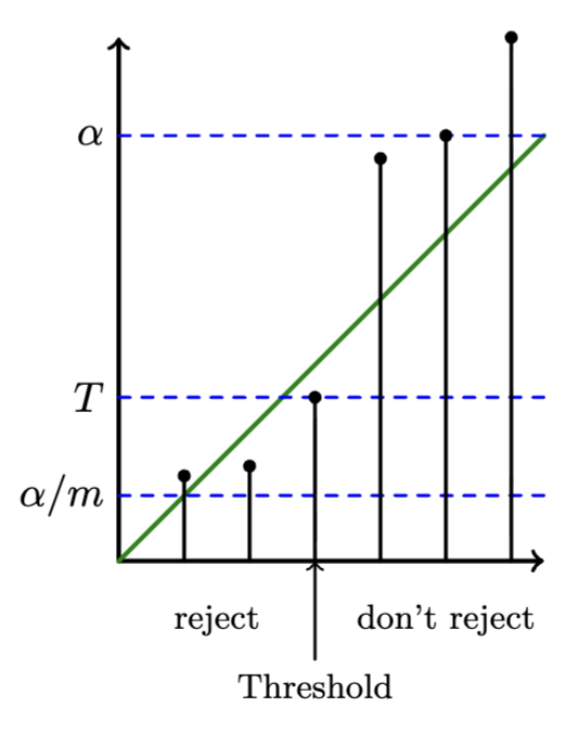
Theorem. (Benjamini-Hochberg Method) After performing all $m$ tests, reject or accept them like so.

First, sort the p-values in non-decreasing order $p_1 \leq p_2 \leq \dots \leq p_m$ .
Identify the greatest index $\ell$ for which $p_{\ell} \leq \ell \cdot \frac{\alpha}{m}$ .
Reject all tests whose p-values are at most $p_{\ell}$ ; that is, reject the tests corresponding to the $\ell$ smallest p-values.

If the test statistics are independent across all $i$ , then $\text{FDR} \leq \alpha$ is guaranteed.

Proof: Say this procedure rejects $R \geq 1$ tests, and say $I_0$ is the set of indices of tests with a true null hypothesis. Then:

\text{FDR} = \mathbb{E}\left[ \frac{\text{\# false positives}}{\text{\# positives}} \right] = \mathbb{E}\left[ \frac{\sum_{i \in I_0} \mathds{1}\left( p_i \leq R \cdot \frac{\alpha}{m} \right)}{R} \right] = \sum_{i \in I_0} \mathbb{E}\left[ \frac{\mathds{1}\left( p_i \leq R \cdot \frac{\alpha}{m} \right)}{R} \right].

If we naively assume $p_i \sim \mathrm{Unif}(0, 1)$ , then the expected value of each term is $\frac{\alpha}{m}$ , yielding $\text{FDR} = \alpha \cdot \frac{|I_0|}{m} \leq \alpha$ .

The logical fallacy here, though, is that $R$ itself is random and dependent on the values of the $p_i$ . The rest of the proof is just working out these technicalities; the explanation above already captures the fundamental essence of the BH method. $\square$

To work around this logical fallacy, here's the trick. For each $i \in I_0$ , let $R_i$ denote the number of tests that would be rejected if $p_i$ were replaced with zero (and all other p-values were kept unchanged).

Lemma 1. It must be that $R_i$ is independent from $p_i$ .

Proof: Obvious, as $R_i$ is by definition a direct function of the values $\{p_j \mid j \neq i\}$ and $\frac{\alpha}{m}$ , which the theorem assumes to be independent of $p_i$ . $\square$

Lemma 2. The following identity is true for all $i \in I_0$ .
$\frac{\mathds{1}\left( {p_i \leq R \cdot \frac{\alpha}{m}} \right)}{R} = \frac{\mathds{1}\left( {p_i \leq R_i \cdot \frac{\alpha}{m}} \right)}{R_i}.$
Proof (Case 1): Suppose that $p_i \leq R \cdot \frac{\alpha}{m}$ . Then $p_i$ is among the $R$ smallest p-values that get rejected. Therefore, replacing $p_i$ with zero only permutes the order of the $R$ smallest p-values, so $R_i = R$ .

Thus, both the LHS and RHS equal $\frac{1}{R} = \frac{1}{R_i}$ , as desired. $\square$

Proof (Case 2): Suppose instead that $p_i > R \cdot \frac{\alpha}{m}$ ; that is, suppose $p_i$ is not rejected. The fact that $p_i$ was not rejected tells us more strongly that $p_i > i \cdot \frac{\alpha}{m}$ .

Note that replacing $p_i$ with zero leaves all p-values with indices above $i$ completely unchanged and unmoved. Therefore, the rejection threshold cannot possibly exceed index $i$ after this change, so $R_i \leq i$ .

Chaining $p_i > i \cdot \frac{\alpha}{m}$ and $R_i \leq i$ together yields $p_i > R_i \cdot \frac{\alpha}{m}$ . Thus, both the LHS and RHS are zero, as desired. $\square$

Lemma 2 lets us freely replace $R$ with $R_i$ in the expression of FDR above, and Lemma 1 gives us the freedom to simplify as we had done naively before.

\text{FDR} = \sum_{i \in I_0} \mathbb{E}\left[ \frac{\mathds{1}\left( p_i \leq R \cdot \frac{\alpha}{m} \right)}{R} \right] = \sum_{i \in I_0} \mathbb{E}\left[ \frac{\mathds{1}\left( p_i \leq R_i \cdot \frac{\alpha}{m} \right)}{R_i} \right] = \sum_{i \in I_0} \frac{\alpha}{m} = \alpha \cdot \frac{|I_0|}{m} \leq \alpha.

And that's the full proof. $\blacksquare$

And so the BH method is better in practice, when we actually expect some of our tests to turn out positive.