MIT 18.701 — Lecture 21

Quaternions, $O_4(\mathbb{R})$ , $SO_4(\mathbb{R})$ , $SO_3(\mathbb{R})$ , and Conjugacy Classes of $SU_2$

§ Quaternion Inner Product and $\{O_4(\mathbb{R}), SO_4(\mathbb{R}), SO_3(\mathbb{R})\}$

Let's continue our discussion of the quaternions $\mathbb{H} = \mathbb{R} \oplus \mathbb{R}i \oplus \mathbb{R}j \oplus \mathbb{R}k$ .

Remark. Think of $\mathbb{H}$ as the vector space $\mathbb{R}^4$ with the additional operation “multiplying two vectors”.

Theorem. (Commutative Real Parts) For any $\alpha, \beta \in \mathbb{H}$ , we have $\Real[\alpha\beta] = \Real[\beta\alpha]$ .

Proof: Say $\alpha = \alpha_1 + \alpha_2i + \alpha_3j + \alpha_4k$ and $\beta = \beta_1 + \beta_2i + \beta_3j + \beta_4k$ . Then just compute. $\blacksquare$

Definition (Quaternion Inner Product). Given $\alpha = \alpha_1 + \alpha_2i + \alpha_3j + \alpha_4k$ and $\beta = \beta_1 + \beta_2i + \beta_3j + \beta_4k$ , their inner product is $\langle \alpha, \beta \rangle := \alpha_1\beta_1 + \alpha_2\beta_2 + \alpha_3\beta_3 + \alpha_4\beta_4 = \mathrm{Re}[\alpha \overline{\beta}]$ . (Check these are equivalent!)

So $\mathbb{H}$ is a four-dimensional Euclidean space. This yields a stronger sense in which $\mathbb{H} \cong \mathbb{R}^4$ . In particular…

Observation. The group of inner-product-preserving linear maps $f: \mathbb{H} \to \mathbb{H}$
is isomorphic to $O_4(\mathbb{R})$ via the usual isomorphism $\mathbb{H} \leftrightarrow \mathbb{R}^4$ .

In particular, $\{1, i, j, k\}$ is an orthonormal basis of $\mathbb{H}$ under this inner product.

To classify these “orthogonal” linear maps $f: \mathbb{H} \to \mathbb{H}$ , we'll need to work with $\mathbb{H}$ and $O_4(\mathbb{R})$ simultaneously!

Theorem. (Quaternions in $O_4(\mathbb{R})$ ) The only inner-product-preserving linear maps $f: \mathbb{H} \to \mathbb{H}$ are $f: x \mapsto \alpha x \beta$ or $f : x \mapsto \alpha \overline{x} \beta$ , for $\alpha, \beta \in \mathbb{H}$ satisfying $|\alpha| = |\beta| = 1$ .

Proof: To show the proposed $f: x \mapsto \alpha x \beta$ works, it suffices to show $f$ maps $\{1, i, j, k\}$ to an orthonormal basis.

\langle f(1), f(i) \rangle = \langle \alpha \beta, \alpha i \beta \rangle = \Real[\alpha\beta \overline{\alpha i \beta} ] = \Real[\alpha \beta \overline{\beta}(-i) \overline{\alpha}] = \Real [ \overline{\alpha} \alpha (-i)] = 0 ~ \text{ since } \overline{\alpha}\alpha \in \mathbb{R}. ~~~~~ \checkmark

(We use $\Real[\alpha \beta ] = \Real [ \beta \alpha ]$ a lot here!) Checking $f: x \mapsto \alpha \overline{x} \beta$ works analogously.

To show these $f$ account for all inner-product-preserving linear maps, we'll need the $\mathbb{H} \leftrightarrow \mathbb{R}^4$ observation.

Claim. All of $O_4(\mathbb{R})$ is generated by reflections.

Proof: From Problem Set #6, we know every element in $O_4(\mathbb{R})$ is the direct sum of two $2 \times 2$ orthogonal submatrices. And $2 \times 2$ orthogonal matrices are generated by reflections. $\square$

It remains to prove the following about reflections:

Claim. Every reflection in $\mathbb{R}^4$ is of the form $f_{\alpha}: x \mapsto - \alpha \overline{x} \alpha$ for some $|\alpha| = 1$ .

Proof: We claim $f_{\alpha}$ is the reflection sending the basis $\{\alpha, \alpha i, \alpha j, \alpha k\}$ to $\{- \alpha, \alpha i, \alpha j, \alpha k\}$ . Indeed,
$f_{\alpha}(\alpha i) = - \alpha \overline{\alpha i} \alpha = - \alpha (-i) \overline{\alpha} \alpha = \alpha i |\alpha |^2 = \alpha i ~~~ \text{ and } ~~~ f_{\alpha}(\alpha) = - \alpha \overline{\alpha} \alpha = - |\alpha|^2 \alpha = -\alpha.$
So $f_{\alpha}$ is a reflection about the hyperplane perpendicular to $\alpha$ . $\square$

Thus, our proposed maps $f: x \mapsto \alpha x \beta$ and $f: x \mapsto \alpha \overline{x} \beta$ include all reflections, which generate $O_4(\mathbb{R})$ ; and they are closed under composition, so they are all of $O_4(\mathbb{R})$ . $\blacksquare$

Remark. Multiplying by elements of $\mathbb{H}$ yields “rotations” of $\mathbb{R}^4$ , whereas conjugation yields “reflections” of $\mathbb{R}^4$ .

In summary, recalling that $\{\alpha \in \mathbb{H} : |\alpha| = 1 \} \cong S^3$ , we have the following description of $O_4(\mathbb{R})$ .

\varphi: S^3 \times S^3 \to O_4(\mathbb{R}) ~ \text{ via } ~ \varphi: (\alpha, \beta) \mapsto \begin{cases} \, (x \mapsto \alpha x \beta) \\ \, (x \mapsto \alpha\overline{x} \beta) \end{cases}

More specifically, one can restrict the above to describe only maps in $SO_4(\mathbb{R})$ .

\varphi: S^3 \times S^3 \to SO_4(\mathbb{R}) ~ \text{ via } ~ \varphi: (\alpha, \beta) \mapsto (x \mapsto \alpha x \beta) ~ \text{ with kernel } ~ \ker \varphi = \{ \pm (1, 1)\}.

This makes sense—conjugations yield “reflections”, which have negative determinant. By corollary…

Theorem. (Describing $SO_3(\mathbb{R})$ ) All rotations of $\mathbb{R} i \oplus \mathbb{R}j \oplus \mathbb{R}k$ are $f: x \mapsto \alpha x \alpha^{-1}$ for $\alpha \in \mathbb{H}$ with $|\alpha| = 1$ .

Proof: Think of $SO_3(\mathbb{R})$ as the subset of $SO_4(\mathbb{R})$ that fixes $1$ . The only maps $(x \mapsto \alpha x \beta)$ that fix $1$ are those for which $\alpha \beta = 1$ , or $\beta = \alpha^{-1}$ . This yields:

\varphi: S^3 \to SO_3(\mathbb{R}) ~ \text{ via } ~ \varphi : \alpha \mapsto (x \mapsto \alpha x \alpha^{-1}) ~ \text{ with kernel } ~ \ker (\varphi) = \{ \pm 1\}.

And that's what we wanted. $\blacksquare$

This is more of a “real-life” application—it implies the following:

Claim. Three-dimensional rotations are parametrized by $S^3 / \{ \pm 1\}$ .

Parametrization: For any $\alpha \in S^3$ , we have a corresponding $\alpha \in \mathbb{H}$ with $|\alpha| = 1$ .
This yields the $\mathbb{H} \to \mathbb{H}$ map defined via $x \mapsto \alpha x \alpha^{-1}$ . Then taking the $(i, j, k)$
components of this $\mathbb{H} \to \mathbb{H}$ map yields a well-defined $\mathbb{R}^3 \to \mathbb{R}^3$ map in $SO_3(\mathbb{R})$ .

Three-dimensional computer graphics use quaternions for this reason!

§ Conjugacy Classes of $SU_2$

Recall from last lecture the following interpretations of $SU_2$ .

\begin{align*}SU_2 \cong \ & \left \{ \left[\begin{smallmatrix} \alpha & \beta \\ - \overline{\beta} & \overline{\alpha} \end{smallmatrix}\right] : \alpha, \beta \in \mathbb{C} \text{ and } |\alpha|^2 + |\beta|^2 = 1\right \} \cong \{v \in \mathbb{R}^4: |v| = 1 \} \cong \{ \alpha \in \mathbb{H} : |\alpha| = 1 \}\cong S^3.\end{align*}

To be more precise about these isomorphisms…

The isomorphism $SU_2 \cong \{v \in \mathbb{R}^4 : |v| = 1\}$ is via $\left[\begin{smallmatrix} \alpha & \beta \\ -\overline{\beta} & \overline{\alpha} \end{smallmatrix}\right] \mapsto (\mathrm{Re}[\alpha], \mathrm{Im}[\alpha], \mathrm{Re}[\beta], \mathrm{Im}[\beta]) \in \mathbb{R}^4$ .
The isomorphism $SU_2 \cong \{ z \in \mathbb{H} : |z| = 1\}$ is via $\left[\begin{smallmatrix} \alpha & \beta \\ -\overline{\beta} & \overline{\alpha} \end{smallmatrix}\right] \mapsto \alpha + \beta j \in \mathbb{H}$ .

Since $SU_2 \cong S^3$ , the previous section showed $SU_2 / \{\pm 1\} \cong SO_3(\mathbb{R})$ ; that is, $SU_2$ is a double cover of $SO_3(\mathbb{R})$ .

Theorem. (Conjugacy Classes of $SU_2$ ) Two matrices in $SU_2$ are conjugate iff they have the same trace.

Proof: To show conjugates always have the same trace, just recall the identity $\mathrm{tr}(XY) = \mathrm{tr}(YX)$ and compute:

\mathrm{tr}(ABA^{-1}) = \mathrm{tr}(A^{-1}AB) = \mathrm{tr}(B).

(More strongly: conjugate matrices always have the same spectra because they're a change-of-basis apart!)

For the other direction, pick some constant $c$ , and consider any $A \in SU_2$ with $\mathrm{tr}(A) = c$ . We wish to show that the condition $\mathrm{tr}(A) = c$ uniquely determines $A$ up to conjugation in $SU_2$ .

By the Spectral Theorem, we have $A = M \Lambda M^{-1}$ for some diagonal matrix $\Lambda$ and some $M \in U_2$ . Well…

Taking $M' := \frac{M}{(\det M)^{1/2}}$ , we see $A = M' \Lambda (M')^{-1}$ for some $M' \in SU_2$ .
Furthermore, we have the following constraints on $\Lambda = \left[\begin{smallmatrix} \lambda_1 & 0 \\ 0 & \lambda_2 \end{smallmatrix}\right]$ .
$\det A = 1 \implies \lambda_1 \lambda_2 = 1 ~~~~~ \text{ and } ~~~~~ \mathrm{tr}(A) = c \implies \lambda_1 + \lambda_2 = c$
Thus, $\{\lambda_1, \lambda_2\}$ is the set of roots $\{r_1, r_2\}$ of $X^2 - cX + 1 = 0$ . In other words, either $\Lambda = \left[\begin{smallmatrix} r_1 & 0 \\ 0 & r_2 \end{smallmatrix}\right]$ or $\Lambda = \left[\begin{smallmatrix} r_2 & 0 \\ 0 & r_1 \end{smallmatrix}\right]$ .

Therefore, any $A \in SU_2$ with $\mathrm{tr}(A) = c$ is conjugate in $SU_2$ to either $\left[\begin{smallmatrix} r_1 & 0 \\ 0 & r_2 \end{smallmatrix}\right]$ or $\left[\begin{smallmatrix} r_2 & 0 \\ 0 & r_1 \end{smallmatrix}\right]$ for fixed constants $\{r_1, r_2\}$ . And these two matrices are conjugates, too (obviously!):

\begin{bmatrix} 0 & -1 \\ 1 & 0 \end{bmatrix} \begin{bmatrix} r_1 & 0 \\ 0 & r_2 \end{bmatrix} \begin{bmatrix} 0 & -1 \\ 1 & 0 \end{bmatrix}^{-1} = \begin{bmatrix} 0 & -1 \\ 1 & 0 \end{bmatrix} \begin{bmatrix} r_1 & 0 \\ 0 & r_2 \end{bmatrix} \begin{bmatrix} 0 & 1 \\ -1 & 0 \end{bmatrix} = \begin{bmatrix} 0 & -1 \\ 1 & 0 \end{bmatrix} \begin{bmatrix} 0 & r_1 \\ -r_2 & 0 \end{bmatrix} = \begin{bmatrix} r_2 & 0 \\ 0 & r_1 \end{bmatrix}.

And so we win. $\blacksquare$

Remark. (Reading Comprehension) In the last step, why did we conjugate by $\left[\begin{smallmatrix} 0 & -1 \\ 1 & 0 \end{smallmatrix}\right]$ instead of $\left[\begin{smallmatrix} 0 & 1 \\ 1 & 0 \end{smallmatrix}\right]$ ?

§ Geometry of $SU_2$ : Latitude and Longitude

Trace in $SU_2$ has a nice analogue in $\mathbb{H}$ , which you can check by plain computation:

Theorem. (Redefining Trace) Every $A = \left[\begin{smallmatrix} \alpha & \beta \\ -\overline{\beta} & \overline{\alpha} \end{smallmatrix}\right] \in SU_2$ yields a $\gamma = \alpha + \beta j \in \mathbb{H}$ . Then $\mathrm{tr}(A) = 2 \mathrm{Re}[\gamma]$ .

This inspires the following geometric description of conjugacy classes in $SU_2$ .

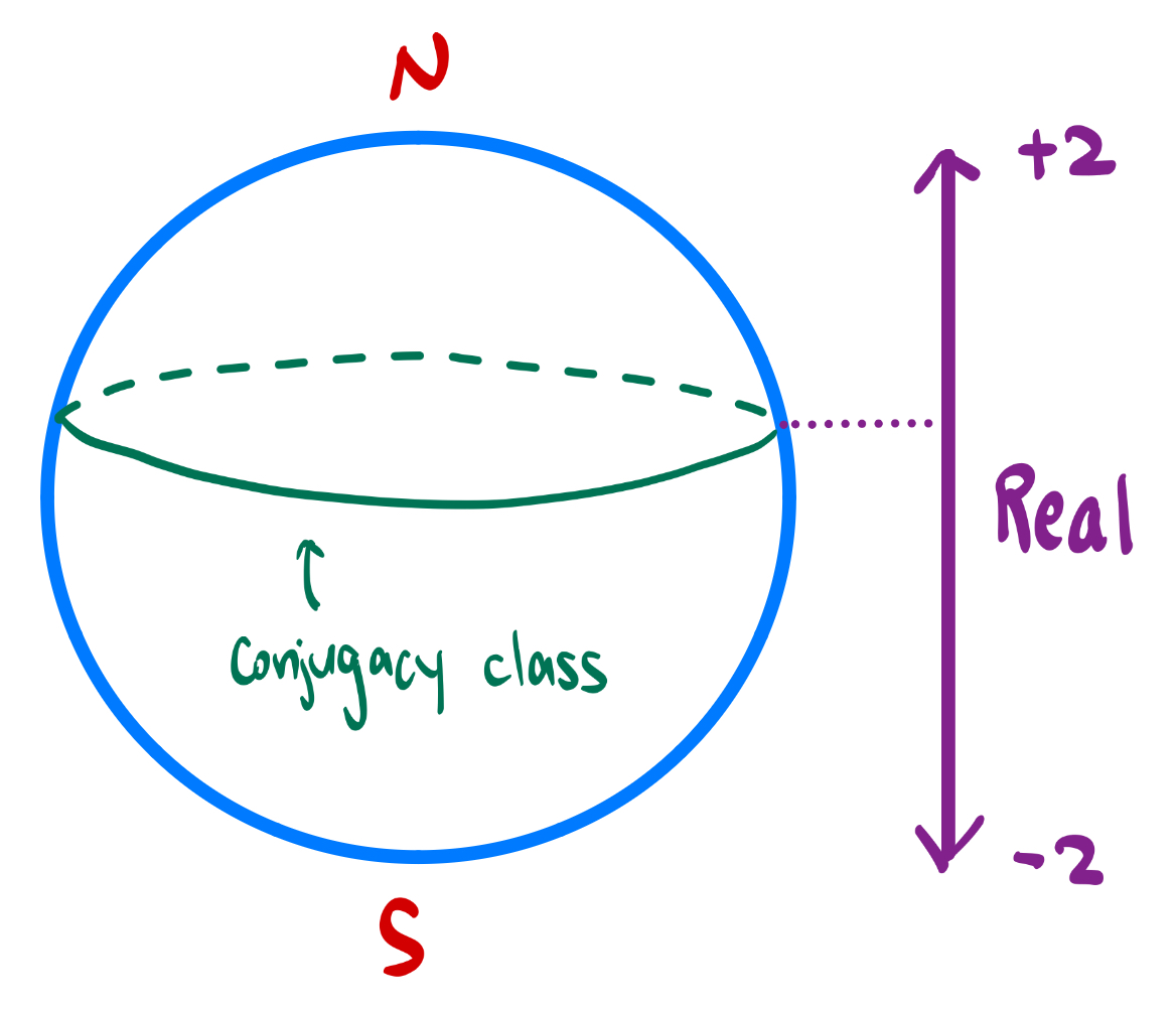
The diagram above has the following features:

The space $SU_2 \cong \{ \alpha \in \mathbb{H} : |\alpha| = 1\} \cong S^3$ is depicted as the blue surface of a sphere.
- Technically speaking, this is wrong! Notably, $S^3$ is the surface of the four-dimensional ball $B^4$ . But we can't draw $B^4$ , so we'll have to settle for using $S^2$ to visually represent $S^3$ .
Conjugacy classes—that is, collections of matrices with the same trace—look like green lines of latitude.

Remark. Keep in mind that everything we say about $SU_2$ applies equally well to the subgroup $\{\alpha \in \mathbb{H} : |\alpha | = 1 \}$ of $\mathbb{H}$ . In particular, multiplication in $SU_2$ is isomorphic to multiplication in $\mathbb{H}$ .

(Reading Comprehension) Convince yourself that the North Pole is $\{+I_2\}$ , and the South Pole is $\{-I_2\}$ .
(Reading Comprehension) Convince yourself that the remaining conjugacy classes of $SU_2$ are isomorphic to $S^2$ .
(Reading Comprehension) Convince yourself that $i$ , $j$ , and $k$ live on the equator of $S^3$ .

We've interpreted the lines of latitude—what about the lines of longitude?

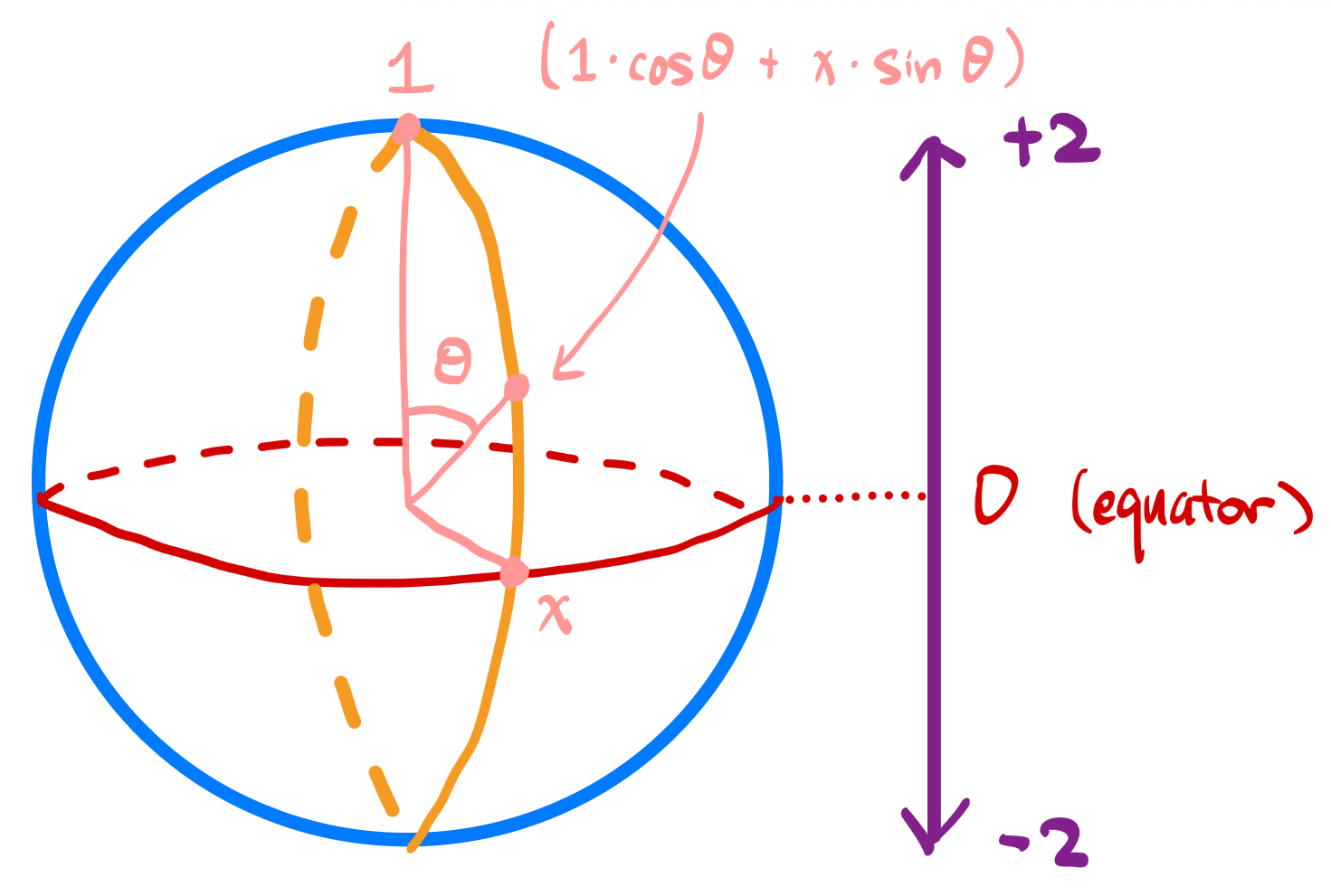
The diagram above has the following features:

The red equator meets the orange line of longitude at some point $x \in S^3$ with $\mathrm{Re}[x] = 0$ .
(Or equivalently, $A \in SU_2$ with $\mathrm{tr}(A) = 0$ .)
The line of longitude is parametrized by $\{ 1 \cdot \cos \theta + x \cdot \sin \theta \mid \theta \in [0, 2\pi) \}$ .

Theorem. (Longitudinal Subgroups) For any $x \in \{ \alpha \in \mathbb{H} : |\alpha| = 1\}$ with $\mathrm{Re}[x] = 0$ , the line of longitude $H_x := \{1 \cdot \cos \theta + x \cdot \sin \theta \mid \theta \in [0, 2\pi)\}$ is a subgroup of $\mathbb{H}$ .

Proof: Both $x \in \mathbb{H}$ and $i \in \mathbb{H}$ lie on the equator, but the equator is a conjugacy class! So $x$ and $i$ are conjugates:

H_x := \{1 \cdot \cos \theta + x \cdot \sin \theta \mid \theta \in [0, 2\pi)\} ~ \text{ is conjugate to } ~ H_i := \{1 \cdot \cos \theta + i \cdot \sin \theta \mid \theta \in [0, 2\pi)\}

But $H_i$ is obviously a subgroup of $\mathbb{H}$ —it's literally just $\{z \in \mathbb{C} : |z| = 1\}$ . $\blacksquare$

§ Geometry of $SU_2$ : Normal Subgroups and Simplicity

One last thing: we'll use the results we've established so far to provide a geometrical proof of the following fact!

Claim. The only normal subgroups of $SU_2$ are $\{1\}$ , $\{1, -1\}$ , and $SU_2$ .

Say $G$ is a normal subgroup of $SU_2$ that is not either $\{1\}$ or $\{1, -1\}$ . We wish to show $G = SU_2$ .

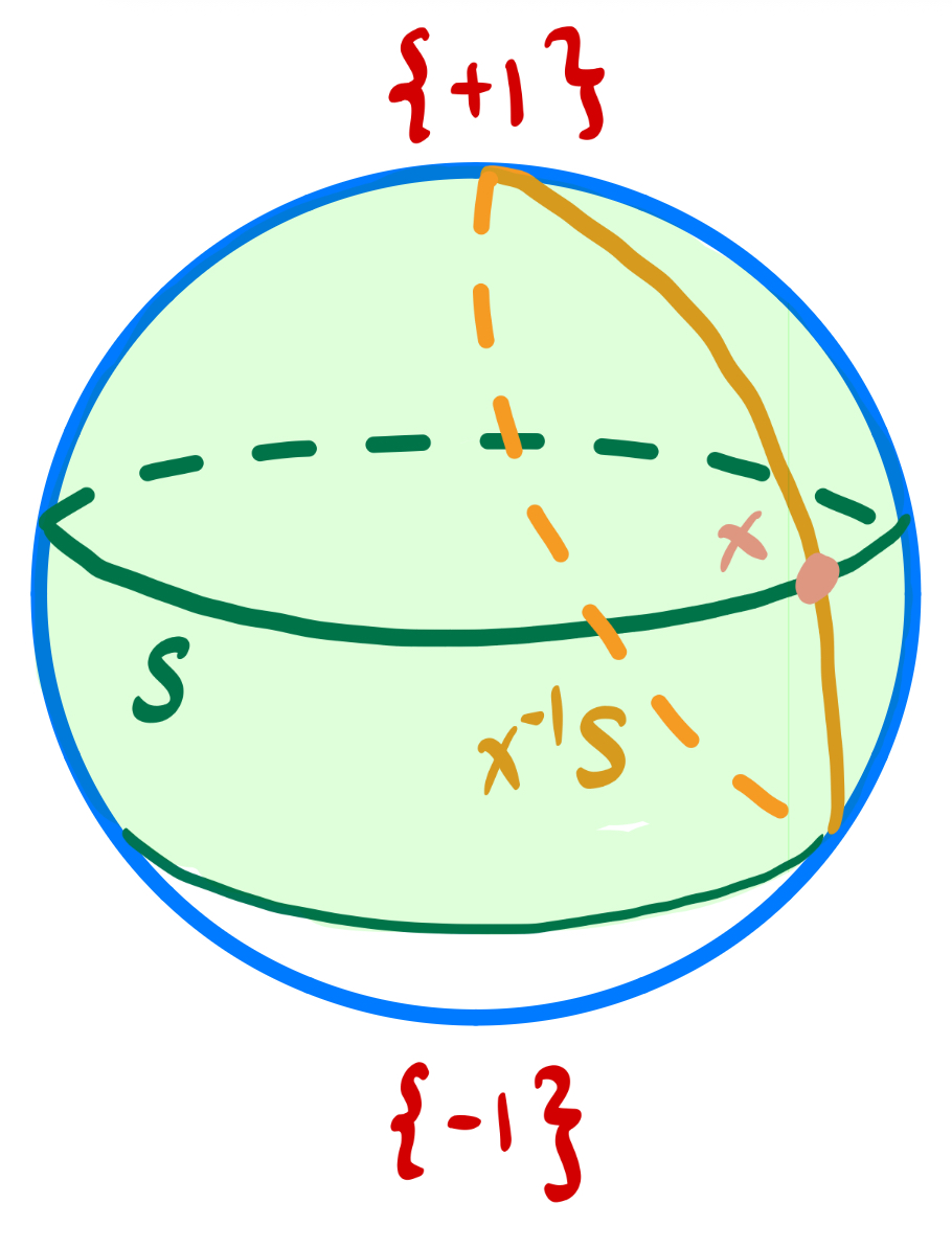
We may pick some $x \in G$ such that $x \not \in \{1, -1\}$ , marked in the diagram below.

The driving principle behind our proof will be the following fact:

Fact. Since $G$ is normal, it is the union of conjugacy classes of $SU_2$ .

Let $S$ be the conjugacy class of $x$ , shown as a green latitudinal line.

Since $x \in G$ , and $G$ is normal, we must also have $S \subseteq G$ .
By closure of groups, we also have $x^{-1}S \subseteq G$ , shown in orange.
Every conjugacy class (highlighted in green) that intersects with an element of $x^{-1}S$ must also be in $G$ .

Thus, just from assuming $x \in G$ , we've shown $G$ must also contain the entire region highlighted in green!

Now consider any longitudinal subgroup $H$ of $SU_2$ . Since $G$ contains the whole region highlighted in green, $G$ must also contain an entire arc of $H$ . And an arc generates all of $H$ , so $H \subseteq G$ .

But the longitudinal subgroups of $SU_2$ together cover all of $SU_2$ . So $G$ contains all of $SU_2$ , done. $\blacksquare$

Remark. By corollary, $SO_3(\mathbb{R}) \cong SU_2 / \{ \pm 1 \}$ is simple.

§ Quaternion Inner Product and {O4(R),SO4(R),SO3(R)}\{O_4(\mathbb{R}), SO_4(\mathbb{R}), SO_3(\mathbb{R})\}{O4​(R),SO4​(R),SO3​(R)}

§ Conjugacy Classes of SU2SU_2SU2​

§ Geometry of SU2SU_2SU2​: Latitude and Longitude

§ Geometry of SU2SU_2SU2​: Normal Subgroups and Simplicity

§ Quaternion Inner Product and $\{O_4(\mathbb{R}), SO_4(\mathbb{R}), SO_3(\mathbb{R})\}$

§ Conjugacy Classes of $SU_2$

§ Geometry of $SU_2$ : Latitude and Longitude

§ Geometry of $SU_2$ : Normal Subgroups and Simplicity