MIT 18.701 — Lecture 22

One-Parameter Subgroups, Lie Algebras, Lie Brackets

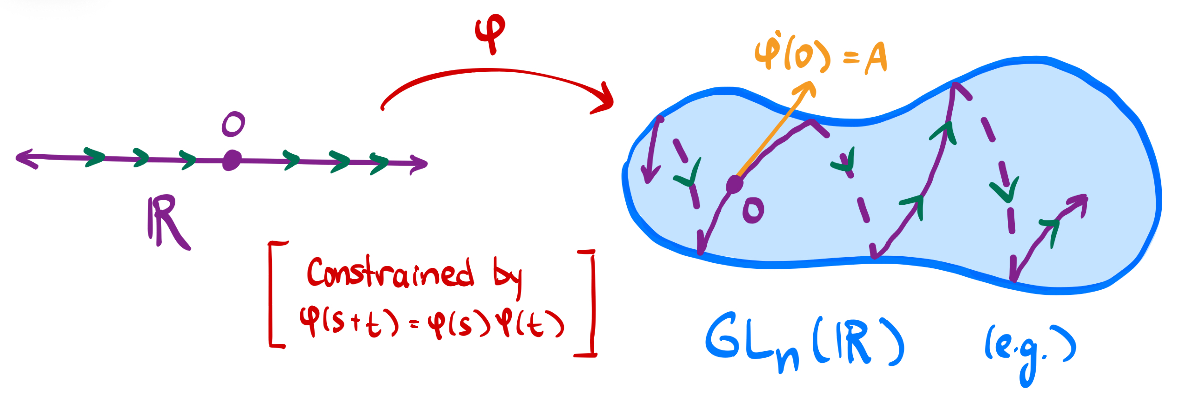
The previous few lectures have prepared us for the following definitions.

Definition (Lie Group). A Lie group is a group that is also a smooth manifold (i.e. looks like $\mathbb{R}^n$ locally).

Example. All of the following are Lie groups: $\{GL_n(\mathbb{R}), GL_n(\mathbb{C}), SO_n, U_n, SU_n\}$ . However, $GL_n(\mathbb{Q})$ is not a Lie group—it has too many “holes” in it.

Definition (One-Parameter Subgroup). Given a Lie group $G$ , a one-parameter subgroup $H \subseteq G$ is a subgroup that is the image of a differentiable homomorphism $\varphi: \mathbb{R} \to G$ .

Example. The longitudinal subgroups from last lecture are one-parameter subgroups of $SU_2$ .

§ Matrix Exponentiation: One-Parameter $GL_n(\mathbb{C})$ Subgroups

Definition (Matrix Exponentiation). Given any $A \in \mathbb{C}^{n \times n}$ , we say $e^A = I_n + A + \frac{A^2}{2!} + \frac{A^3}{3!} + \dots$ (Taylor Series).

Theorem. (Exponent Laws) For any $A, B \in \mathbb{C}^{n \times n}$ such that $AB = BA$ , we have $e^{A + B} = e^A e^B$ .

Proof: Apply the distributive law to $e^Ae^B = \left(\sum_{k \geq 0} \frac{A^k}{k!}\right)\left(\sum_{\ell \geq 0} \frac{B^{\ell}}{\ell!}\right)$ , where $AB = BA$ lets us collate factors together.

Really, this theorem is just restating $(x + y)^n = \sum_{k = 0}^n \binom{n}{k}x^ky^{n - k}$ , which only holds when $x$ and $y$ commute. $\blacksquare$

To actually compute the exponentiation by a matrix, use diagonalizability.

Theorem. (Diagonalizable Computations) If $A$ is diagonalizable, then we have:

A = B \left[\begin{smallmatrix} \lambda_1 & \cdots & 0 \\ \vdots & \ddots & \vdots \\ 0 & \cdots & \lambda_n \end{smallmatrix}\right]B^{-1} ~~~ \implies ~~~ e^A = B \left[\begin{smallmatrix} e^{\lambda_1} & \cdots & 0 \\ \vdots & \ddots & \vdots \\ 0 & \cdots & e^{\lambda_n} \end{smallmatrix}\right] B^{-1}.

In fact, most matrices are diagonalizable, so…

Theorem. (Determinant and Trace) For any $A \in \mathbb{C}^{n \times n}$ , we have $\det e^A = e^{\mathrm{tr}(A)}$ .

Proof: This holds when $A$ is diagonalizable. By continuity, it holds for all $A$ . $\blacksquare$

The point of all this setup is the following observation:

Observation. For any $A \in \mathbb{C}^{n \times n}$ , the map $\varphi_A: \mathbb{R} \to GL_n(\mathbb{C})$ via $\varphi_A(s) = e^{sA}$ yields a one-parameter subgroup of $GL_n(\mathbb{C})$ .

In particular, the derivative is $\frac{d}{ds} \varphi_A(s) = A \varphi_A(s)$ .

Remark. (Reading Comprehension) Why is $\varphi_A(s) = e^{sA} \in GL_n(\mathbb{C})$ always true for any $A \in \mathbb{C}^{n \times n}$ ?

And here's an even stronger observation.

Theorem. (One-Parameter General Subgroups) Suppose $\varphi : \mathbb{R} \to GL_n(\mathbb{C})$ yields a one-parameter subgroup of $GL_n(\mathbb{C})$ . Then $\varphi$ looks like $\varphi: s \mapsto e^{As}$ for some $A \in \mathbb{C}^{n \times n}$ .

Proof: This is effectively a functional equation, with constraints:

(1) ~~ \varphi(0) = I_n ~~~~~~~ (2) ~~ \varphi(s + t) = \varphi(s) \varphi(t)

Differentiating (2) and taking $s = 0$ yields $\varphi'(t) = \varphi'(0) \varphi(t)$ . Say $A = \varphi'(0)$ . The point is that $\varphi'(t) = A \varphi(t)$ is a linear first-order ODE, so it has a unique solution satisfying (1), and $\varphi: t \mapsto e^{tA}$ is such a solution. $\blacksquare$

Remark. Recall the only solution to Cauchy's FE—provided $f$ is continuous!—is the linear equation.

One can think of every one-parameter subgroup of $GL_n(\mathbb{C})$ as being parametrized by its “tangent vector” $\varphi'(0)$ . Once the “initial conditions” $\varphi(0) = I_n$ and $\varphi'(0) = A$ are set, the rest of the path is fixed!

§ One-Parameter Subgroups of $SL_n(\mathbb{C})$ and $O_n(\mathbb{R})$

More generally, for any subgroup $G \subseteq GL_n(\mathbb{C})$ , the one-parameter subgroups of $G$ are precisely the images of maps $\varphi: \mathbb{R} \to G$ via $\varphi : s \mapsto e^{As}$ for some $A \in \mathbb{C}^{n \times n}$ . The only constraint on $A$ is that $e^{As} \in G$ for all $s \in \mathbb{R}$ .

Let's investigate this constraint for various $G \subseteq GL_n(\mathbb{C})$ .

Theorem. (One-Parameter Special Subgroups) The one-parameter subgroups of $SL_n(\mathbb{C})$ are precisely the images of $\varphi: s \mapsto e^{sA}$ for some $A \in \mathbb{C}^{n \times n}$ satisfying $\mathrm{tr}(A) = 0$ .

Proof: We just need $e^{sA} \in SL_n(\mathbb{C})$ for all $s \in \mathbb{R}$ , or:

\det e^{sA} = 1 ~ \implies ~ 1 = \det e^{sA} = e^{\mathrm{tr}(sA)} = e^{s \cdot \mathrm{tr}(A)}.

And the above could only hold for all $s$ if $\mathrm{tr}(A) = 0$ . $\blacksquare$

Similarly, we can talk about one-parameter subgroups of $O_n(\mathbb{R})$ .

Theorem. (One-Parameter Orthogonal Subgroups) The one-parameter subgroups of $O_n(\mathbb{R})$ are precisely the images of $\varphi: s \mapsto e^{sA}$ for some $A \in \mathbb{R}^{n \times n}$ satisfying $A^{\top} = -A$ (i.e. skew-symmetric matrices).

Proof: We just need $e^{sA} \in O_n(\mathbb{R})$ for all $s \in \mathbb{R}$ , or:

I_n = e^{sA}(e^{sA})^{\top} = e^{sA} e^{s A^{\top}}.

Differentiating at $s = 0$ forces $A + A^{\top} = 0$ , so $A^{\top} = -A$ . $\blacksquare$

The one-parameter subgroups of $O_n(\mathbb{R})$ actually tell us about its dimension!

Theorem. (Dimension of Orthogonal Subgroups) We have $\dim O_n(\mathbb{R}) = \binom{n}{2}$ .

Proof: It's equivalent to know the dimension of the set of one-parameter subgroups of $O_n(\mathbb{R})$ . But these biject with the set of skew-symmetric matrices, which is of dimension $\binom{n}{2}$ . $\blacksquare$

Remark. This is pretty hard to show without inspecting the one-parameter subgroups!

Note that if $\varphi: s \mapsto e^{sA}$ describes a one-parameter subgroup of $G$ , we need not have $A \in G$ . For example, $A = \left[\begin{smallmatrix} 1 & 0 \\ 0 & -1 \end{smallmatrix}\right]$ generates a one-parameter subgroup of $SL_2(\mathbb{C})$ , but $\left[\begin{smallmatrix} 1 & 0 \\ 0 & -1 \end{smallmatrix}\right]$ is not in $SL_2(\mathbb{C})$ . We only need $A \in \mathbb{C}^{n \times n}$ .

Remark. (Reading Comprehension) Show that the one-parameter subgroups of $SU_2$ are precisely the images of $\varphi: s \mapsto e^{sA}$ for some $A \in \mathbb{C}^{n \times n}$ satisfying $A^{\dagger} = -A$ and $\mathrm{tr}(A) = 0$ . For example, $A = \left[\begin{smallmatrix} i & -6 \\ 6 & -i \end{smallmatrix}\right]$ works.

If $A \in \mathbb{C}^{n \times n}$ does not satisfy this, then the path $\varphi(s) := e^{sA}$ will “fly off” the surface $S^3$ .

§ Lie Algebras and Lie Brackets

Definition (Lie Algebra). If $G$ is a Lie group, then its Lie algebra $\mathrm{Lie}(G)$ is the tangent space at its identity—in other words, the set of all possible $\varphi'(0)$ for one-parameter subgroups $\varphi: \mathbb{R} \to G$ .

Definition (Lie Bracket). Every Lie algebra of matrices is equipped with the Lie bracket $[A, B] := AB - BA$ .

Example. The Lie algebra of $SL_n(\mathbb{C})$ is $\{A \in \mathbb{C}^{n \times n} : \mathrm{tr}(A) = 0\}$ , and that of $O_n(\mathbb{R})$ is $\{ A \in \mathbb{R}^{n \times n} : A^{\top} = -A \}$ . Meanwhile, the Lie algebra of $GL_n(\mathbb{C})$ is just all of $\mathbb{C}^{n \times n}$ .

In the specific case of matrix groups, we have the following alternative definition:

Definition (Lie Algebra). If $G \subseteq GL_n(\mathbb{C})$ is a Lie group, then its Lie algebra is:

\mathrm{Lie}(G) := \{ A \in \mathbb{C}^{n \times n} \mid e^{sA} \in G \text{ for all } s \in \mathbb{R}\}.

Let's check some closure properties of Lie algebras and the Lie bracket.

Theorem. (Closure of Addition) For any $A, B \in \mathrm{Lie}(G)$ , we have $A + B \in \mathrm{Lie}(G)$ .

Proof: The fact that $A, B \in \mathrm{Lie}(G)$ is equivalent to the fact that $e^{sA}$ and $e^{sB}$ are in $G$ for all $s \in \mathbb{R}$ . Therefore, their product $e^{sA}e^{sB} = I_n + (A + B)s + O(s^2)$ is in $G$ for all $s \in \mathbb{R}$ , so $A + B$ is a valid direction in the tangent space at the identity, meaning $A + B \in \mathrm{Lie}(G)$ . $\blacksquare$

Theorem. (Closure of Lie Bracket) For any $A, B \in \mathrm{Lie}(G)$ , we have $[A, B] \in \mathrm{Lie}(G)$ .

Proof: The idea is to consider the following expression:

\begin{align*}e^{As} e^{Bs} e^{-As} e^{-Bs} = \ & \left(1 + As + \frac{A^2s^2}{2} + O(s^3) \right) \left(1 + Bs + \frac{B^2s^2}{2} + O(s^3) \right)\left(\dots \text{$e^{-As}$}\dots \right)\left(\dots \text{$e^{-Bs}$}\dots \right) \\ = \ & 1 + (AB - BA)s^2 + O(s^3) ~ \text{ after much simplification.}\end{align*}

The above is in $G$ for all $s \in \mathbb{R}$ . Thus, sending $s \to 0$ , we see $e^{s^2(AB - BA)}$ is in $G$ . Therefore, “locally” speaking, $AB - BA$ is a valid direction in the tangent space at the identity, so $AB - BA = [A, B]$ is in $\mathrm{Lie}(G)$ . $\blacksquare$

Remark. It is not the case that $A, B \in \mathrm{Lie}(G)$ implies $AB \in \mathrm{Lie}(G)$ . (Try to find a counterexample!)

The Lie Bracket also has a bunch of identities, which one can check if they really want to.

Theorem. (Lie Bracket Identities) The following identities are true for any $A, B, C \in \mathrm{Lie}(G)$ and $c \in \mathbb{R}$ .

(1) ~~ [A + B, C] = [A, C] + [B, C] ~~~~~ (2) ~~ [cA, B] = c[A, B] ~~~~~ (3) ~~ [A, B] = -[B, A]

(4) ~~ [A, [B, C]] + [B, [C, A]] + [C, [A, B]] = 0

Remark. Identity (4) is known as the Jacobi Identity, equivalent to $[A, [B, C]] = [[A, B], C] + [B, [A, C]]$ .

There's a neat analogy to the product rule $\frac{d}{dt} \left [ f(t) g(t) \right ] = \left [ \frac{d}{dt}f(t) \right ] g(t) + f(t) \left [ \frac{d}{dt} g(t) \right ]$ .

Every Lie group has a corresponding Lie algebra, found via “differentiation”. However, just as “integration” always has a $+C$ term, not every Lie algebra has a unique Lie group; uniqueness is only guaranteed up to coverings.

Example. Both $\mathbb{R}$ and $S^1$ have isomorphic Lie algebras, and $\mathbb{R} / \mathbb{Z} \cong S^1$ indicates their mutual covering group.

We care about Lie algebras because they turn geometry and physics problems (i.e. Lie groups) into linear algebra problems (i.e. Lie algebras).

§ Matrix Exponentiation: One-Parameter GLn(C)GL_n(\mathbb{C})GLn​(C) Subgroups

§ One-Parameter Subgroups of SLn(C)SL_n(\mathbb{C})SLn​(C) and On(R)O_n(\mathbb{R})On​(R)

§ Lie Algebras and Lie Brackets

§ Matrix Exponentiation: One-Parameter $GL_n(\mathbb{C})$ Subgroups

§ One-Parameter Subgroups of $SL_n(\mathbb{C})$ and $O_n(\mathbb{R})$