MIT 6.300 — Lecture 10

Frequency Response and Filtering

§ Lecture: Frequency Response

Theorem. (Complex Exponential Convolution) Consider an LTI system given by $x[n] \mapsto (x * h)[n]$ . Suppose the Fourier transform of $h[n]$ is $H(\Omega)$ . Then the system sends $e^{j\Omega n} \mapsto H(\Omega) e^{j\Omega n}$ .

The same goes for CT signals: if the Fourier transform of $h(t)$ is $H(\omega)$ , then the system sends $e^{j\omega t} \mapsto H(\omega) e^{j\omega t}$ .

Proof: Just follow what the convolution does (reindexing $m \to n - m$ along the way).

e^{j\Omega n} ~~~\mapsto ~~~ \sum_{m = -\infty}^{\infty} e^{j\Omega (n - m)} h[m] = e^{j\Omega n} \left[ \sum_{m = -\infty}^{\infty} h[m] e^{-j\Omega m} \right] = e^{j\Omega n} \left[ H(\Omega) \right].

That last step is just the definition of the Fourier transform. The argument looks identical for CT signals. $\blacksquare$

Definition. The Fourier transform $H(\Omega)$ / $H(\omega)$ of the unit-sample / impulse response is called the frequency response.

Remark. Complex exponentials are eigenfunctions of LTI systems, and the frequency response $H(\Omega)$ is the eigenvalue.

Problem. Determine the response of an LTI system to the input $x[n] = \cos(\Omega n)$ , based on the unit-sample response $h[n]$ and its Fourier transform $H(\Omega)$ . Assume all signals are real-valued.

Solution: The point is that $x[n] = \frac{1}{2}\left(e^{j \Omega n} + e^{-j \Omega n}\right)$ and that LTI systems are linear. The preceding theorem thus gives:

\cos(\Omega n) ~~~ \mapsto ~~~ \frac{1}{2}\left(H(\Omega) e^{j \Omega n} + H(-\Omega) e^{-j \Omega n}\right).

Since $h[n]$ is real, we furthermore know $H(-\Omega) = \overline{H(\Omega)}$ (Hermitian symmetry). So the two terms above are conjugates of each other, allowing us to simplify further:

\frac{1}{2}\left(H(\Omega) e^{j \Omega n} + \overline{H(\Omega)} e^{-j \Omega n}\right) = \mathrm{Re}\left[H(\Omega) e^{j \Omega n}\right] = |H(\Omega)| \cos\left(\Omega n + \angle H(\Omega)\right).

In the above, $\angle H(\Omega)$ denotes the phase of $H(\Omega)$ .

§ Lecture: LTIs by Frequency Response

Last lecture, we saw that every LTI system could be defined by a single unit-sample / impulse response. This lecture, we see that another natural way to define LTI systems is by their frequency response.

Theorem. (LTI = Frequency Multiplication) Consider an LTI system $x[n] \mapsto (x * h)[n]$ . Then if $x[n]$ has response $y[n]$ , we have $Y(\Omega) = H(\Omega) \cdot X(\Omega)$ . In other words, the Fourier transform of a convolution is the product of Fourier transforms.

Proof: There's actually nothing new here. Just combine the following two observations:

Complex exponentials $e^{j\Omega n}$ get multiplied by $H(\Omega)$ under any LTI system.
All DT signals are just linear combinations of complex exponentials.

Then the linearity of LTI systems finishes the proof.

Warning: The eigenvalue $H(\Omega)$ is not a constant; different eigenfunctions have different eigenvalues!

If $x[n]$ is a single eigenfunction—say, $x[n] := e^{2j n}$ — then passing $x[n]$ through an LTI system is the same as scaling $x[n]$ by $H(\Omega)$ —in this case, $y[n] = H(2) \cdot e^{2jn}$ .

But in any other case, passing $x[n]$ through an LTI system is not as easy as just scaling $x[n]$ by $H(\Omega)$ . Each eigenfunction that makes up $x[n]$ gets scaled by its own scalar $H(\Omega)$ , so the net effect on $x[n]$ is not that simple.

Written out explicitly, the proof would look like this:

\begin{align*}Y(\Omega) & = \sum_{n = -\infty}^{\infty} y[n] \cdot e^{-j\Omega n} \\ & = \sum_{n = -\infty}^{\infty} \left( \sum_{m = -\infty}^{\infty} x[m] \cdot h[n - m] \right) \cdot e^{-j\Omega n} ~~~ \text{ because } y = x * h \\ & = \sum_{m = -\infty}^{\infty} x[m] \cdot \left( \sum_{n = -\infty}^{\infty} h[n - m] \cdot e^{-j \Omega n} \right) ~~~ \text{ by swapping the order of summation} \\ & = \sum_{m = -\infty}^{\infty} x[m] \cdot \left( \sum_{n' = -\infty}^{\infty} h[n'] e^{-j\Omega(n' + m)} \right) ~~~ \text{ by reparametrizing } n' = n - m \\ & = \left(\sum_{m = -\infty}^{\infty} x[m] e^{-j \Omega m}\right) \cdot \left(\sum_{n' = -\infty}^{\infty} h[n'] e^{-j\Omega n'}\right) = X(\Omega) H(\Omega).\end{align*}

But really, this is just a more-syntactically-involved version of the proof of the “Complex Exponential Convolution” theorem. $\blacksquare$

Problem. An LTI system $x[n] \mapsto y[n]$ satisfies $y[n] - \alpha y[n - 1] = x[n]$ , where $|\alpha| < 1$ . It is also initially at rest: if $x[n] = 0$ for all $n < 0$ , then $y[n] = 0$ for all $n < 0$ . Find the frequency response.

Solution: We present three different approaches. The first is to solve for the unit-sample response and take its Fourier transform.

Solution 1. Taking the input $x[n]$ to be the unit-sample signal $\delta[n]$ , we find its response to be:
$h[n] = \begin{cases} \alpha^n & \text{ for all } n \geq 0. \\ 0 & \text{ for all } n < 0. \end{cases} \implies H(\Omega) = \sum_{n = -\infty}^{\infty} h[n] e^{-j \Omega n} = \frac{1}{1 - \alpha e^{-j \Omega}}.$

Another approach is to find the response of $e^{j \Omega n}$ directly.

Solution 2. Taking the input $x[n]$ to be $e^{j \Omega n}$ , we expect the output $y[n]$ to be $H(\Omega) e^{j \Omega n}$ . Therefore,
$H(\Omega) e^{j \Omega n} - \alpha H(\Omega) e^{j \Omega (n - 1)} = e^{j \Omega n} ~~~ \implies ~~~ H(\Omega) - \alpha H(\Omega) e^{-j \Omega} = 1 ~~~ \implies ~~~ H(\Omega) = \frac{1}{1 - \alpha e^{-j \Omega}}.$

The third solution is to take the Fourier transform of the given relationship.

Solution 3. Given $y[n] - \alpha y[n - 1] = x[n]$ , the Fourier transform of the LHS must equal that of the RHS, so:
$Y(\Omega) - \alpha e^{-j \Omega} Y(\Omega) = X(\Omega) ~~~ \implies ~~~ Y(\Omega) = \left(\frac{1}{1 - \alpha e^{-j \Omega}}\right) X(\Omega) ~~~ \implies ~~~ H(\Omega) = \frac{1}{1 - \alpha e^{-j \Omega}}.$

As expected, all three solutions give the same answer.

§ Recitation: Filter Types

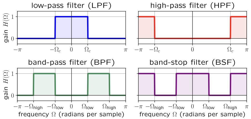
Pictured below are the frequency responses of four filter types: low-pass, high-pass, band-pass, and band-stop.

Convolving a signal with such an (ideal) filter will leave some of its frequencies unchanged and completely zero out other frequencies. (Realistic filters, like the ones later this lecture, only attenuate the frequencies they reject.)

Problem. Consider an ideal low-pass DT-signal filter that only accepts frequencies below $\Omega_c$ . Determine $h[n]$ for this filter.

Solution: The frequency response $H(\Omega)$ looks like this:

H(\Omega) = \begin{cases} 1 & \text{ if } \Omega \in (-\Omega_c, \Omega_c) \\ 0 & \text{ otherwise. } \end{cases}

Since $H(\Omega)$ is the Fourier transform of $h[n]$ , we have:

h[n] = \frac{1}{2\pi} \int_{-\pi}^\pi H(\Omega) e^{j \Omega n} \, \mathrm{d}\Omega = \frac{1}{2\pi} \int_{-\Omega_c}^{\Omega_c} e^{j \Omega n} \, \mathrm{d}\Omega = \frac{\sin(\Omega_c n)}{\pi n}.

(At $n = 0$ , interpret this formula by its limit: $h[0] = \frac{\Omega_c}{\pi}$ .)

§ Lecture: Identifying Filters

More generally, we can study the highs and lows of an LTI system's frequency response to determine what kind of filter it is.

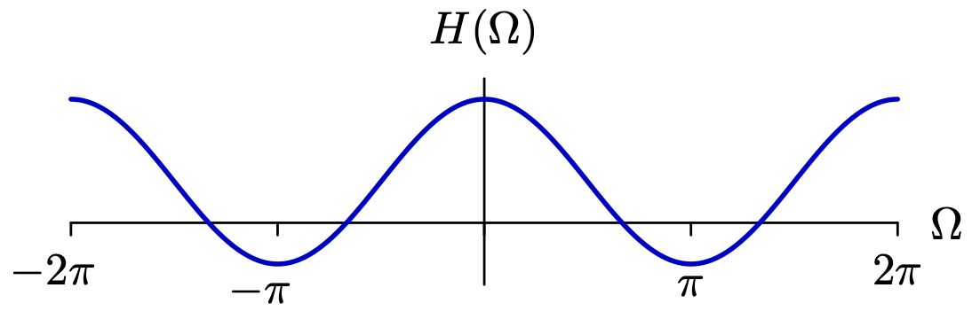
Problem. Determine the frequency response of $y[n] = \frac{1}{3}(x[n - 1] + x[n] + x[n + 1])$ . Is this a low-pass filter?

Solution: Using any approach you'd like (try all three in your head!), we discover that:

H(\Omega) = \frac{1}{3} e^{j \Omega} + \frac{1}{3} + \frac{1}{3} e^{-j \Omega} = \frac{1}{3}\left(1 + 2\cos(\Omega)\right).

The graph of $H(\Omega)$ is shown below.

A reminder on DT signals and their Fourier transforms:

Because $e^{j\Omega n} = e^{j(\Omega \pm 2\pi) n}$ , we can take all frequencies $\Omega$ modulo $2\pi$ , meaning we may assume $\Omega \in (-\pi, \pi]$ .
Assuming $h[n]$ is real, the behavior of $H(\Omega)$ over $(-\pi, 0)$ must be the conjugate of that over $(0, \pi)$ .

Therefore, it suffices only to investigate the behavior of $H(\Omega)$ over the “baseband” interval $\Omega \in [0, \pi]$ . Low frequencies are those close to $0$ , and high frequencies are those close to $\pi$ .

This is not a low-pass filter; it does not filter out high frequencies.

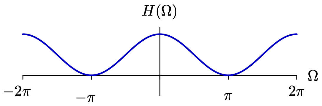
Problem. Determine the frequency response of $y[n] = \frac{1}{4}(x[n - 1] + 2x[n] + x[n + 1])$ . Is it a low-pass filter?

Solution: Again, using any approach you'd like, we discover that:

H(\Omega) = \frac{1}{4}e^{j \Omega} + \frac{1}{2} + \frac{1}{4}e^{-j \Omega} = \frac{1}{2}\left(1 + \cos(\Omega)\right).

The graph of $H(\Omega)$ is shown below.

This is a low-pass filter, since $H(\Omega)$ is close to zero for large frequencies $\Omega$ close to $\pi$ .

Remark. Given the frequency response $H(\Omega) = \frac{1}{1 - \alpha e^{-j \Omega}}$ , argue that the following are true, assuming $\alpha \in (0, 1)$ .

Low baseband frequencies are amplified, whereas high baseband frequencies are attenuated.
Both low and high baseband frequencies are delayed.

(This requires studying not just the magnitude of the frequency response, but its phase as well.)

§ Lecture: Frequency Response for CT Signals

By identical arguments, everything stated above applies just as well to CT signals.

Theorem. (LTI = Frequency Multiplication) Consider an LTI system with frequency response $H(\omega)$ . If the CT signal $x(t)$ has response $y(t)$ , then $Y(\omega) = H(\omega) \cdot X(\omega)$ .

Problem. An LTI system $x(t) \mapsto y(t)$ satisfies $y(t) + \alpha \frac{d}{dt} y(t) = 2x(t)$ . Find the frequency response.

Solution: We present two different approaches. The first is to find the response of $e^{j \omega t}$ directly.

Solution 1. Taking the input $x(t)$ to be $e^{j \omega t}$ , we expect the output $y(t)$ to be $H(\omega) e^{j \omega t}$ . Therefore,
$H(\omega) e^{j \omega t} + j \omega \alpha H(\omega) e^{j \omega t} = 2 e^{j \omega t} ~~~ \implies ~~~ H(\omega) + j \omega \alpha H(\omega) = 2 ~~~ \implies ~~~ H(\omega) = \frac{2}{1 + j \omega \alpha}.$

The second approach is to take the Fourier transform of the given relationship.

Solution 2. Given $y(t) + \alpha \frac{d}{dt} y(t) = 2x(t)$ , the Fourier transform of the LHS must equal that of the RHS, so:
$Y(\omega) + j \omega \alpha Y(\omega) = 2 X(\omega) ~~~ \implies ~~~ Y(\omega) = \left(\frac{2}{1 + j \omega \alpha}\right) X(\omega) ~~~ \implies ~~~ H(\omega) = \frac{2}{1 + j \omega \alpha}.$

Taking $x(t)$ to be $\delta(t)$ is not one of these solutions; it's too clunky.

Remark. Given the frequency response $H(\omega) = \frac{2}{1 + j \omega \alpha}$ , argue that the following are true, assuming $\alpha \in (0, 1)$ .

Low frequencies are amplified, whereas high frequencies are attenuated.
Both low and high frequencies are delayed.

§ Recitation: Cascaded Systems

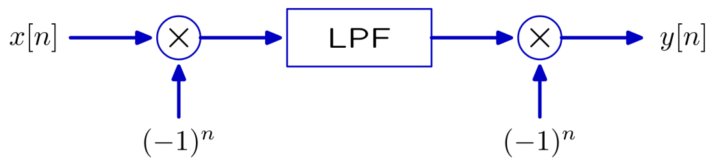
Consider the cascaded system below. It is the composition of three systems: one of which is a low-pass filter, and two of which are the maps $x[n] \mapsto (-1)^n \cdot x[n]$ .

Interestingly, we may note the following:

The maps $x[n] \mapsto (-1)^n \cdot x[n]$ are linear but not time-invariant.
The low-pass filter is linear and time-invariant. (It's an LTI system.)
The cascaded system, altogether, is both linear and time-invariant!
The cascaded system is a high-pass filter (HPF). Here's why.

Proof: Say the LPF has a unit-sample response of $h[n]$ . Then:
$y[n] = (-1)^n \cdot \sum_{m = -\infty}^{\infty} (-1)^m \cdot x[m] h[n - m] = \sum_{m = -\infty}^{\infty} x[m] \underbrace{\left[ (-1)^{n - m}h[n - m] \right]}_{ h'[n - m] }.$
So the cascaded system has a unit-sample response of $h'[n] := (-1)^n h[n] = e^{j \pi n} h[n]$ . Therefore, $H'(\Omega) = H(\Omega - \pi)$ (plug $h'[n]$ into the analysis equation to check).

Graphically, this means that the accepted band of low frequencies in $H(\Omega)$ gets translated to become an accepted band of high frequencies in $H'(\Omega)$ , so this is an HPF.