MIT 6.300 — Lecture 7

DT Fourier Transform

§ Lecture: The DT Fourier Transform

Let's do it all again for DT. You might take the following as a prototypical example.

f[n] := \begin{cases} 1 & \text{ if } n \in \{-2, -1, 0, 1, 2\}. \\ 0 & \text{ otherwise.} \end{cases}

The goal, as before, is to express $f[n]$ as a sum (or rather, integral) of complex exponentials, even though $f[n]$ is aperiodic.

We'll just cut straight to the punchline this time.

Theorem. (DT Fourier Transform) Given a DT signal $f[n]$ , define its Fourier transform to be $F(\Omega) := \sum_{n = -\infty}^{\infty} f[n] e^{-j \Omega n}$ . It then follows that $f[n] = \frac{1}{2\pi} \int_{0}^{2\pi} F(\Omega) e^{j \Omega n} \, \mathrm{d}\Omega$ .

Remark. Even though the signal $f[n]$ is discrete and possibly aperiodic, the Fourier transform $F(\Omega)$ is continuous and guaranteed periodic with period $2\pi$ .

Proof: Our strategy is the same as last time: consider signals $f_N[n]$ that are extensions of $f[n]$ to have period $N$ , take the DT Fourier series of $f_N[n]$ , and investigate the series for $N \to \infty$ .

The DT Fourier series for $f_N[n]$ looks like:

f_N[n] = \sum_{k \in \langle N \rangle} F_N[k] e^{jn \textcolor{#bf0140}{(2\pi k / N)}} ~ \text{ where } ~ F_N[k] = \frac{1}{N} \sum_{n \in \langle N \rangle} f_N[n] e^{-jn \textcolor{#bf0140}{(2\pi k / N)}}.

Here, $\langle N \rangle$ denotes a set of $N$ consecutive integers roughly centered at zero. Remember that for DT Fourier series, $F_N[k]$ is a finite array of length $N$ , or equivalently, an infinite array with period $N$ .

Let's follow the recipe from last time: take $F(\Omega) := \lim_{N \to \infty} N \cdot F_N[k]$ , where the continuous frequency variable $\textcolor{#bf0140}{\Omega := 2\pi k / N}$ is held fixed as $N \to \infty$ (so the index $k$ grows in proportion to $N$ ). Then:

F(\Omega) = \lim_{N \to \infty} N \cdot \left( \frac{1}{N} \sum_{n \in \langle N \rangle} f_N[n] e^{-jn \textcolor{#bf0140}{(2\pi k / N)}} \right) = \lim_{N \to \infty} \sum_{n \in \langle N \rangle} f_N[n] e^{-jn \textcolor{#bf0140}{\Omega}} = \sum_{n = -\infty}^{\infty} f[n] e^{-jn \textcolor{#bf0140}{\Omega}}.

Just as promised. Now make the parametrization $\{\Omega_k\}_{k \in \langle N \rangle}$ where $\textcolor{#bf0140}{\Omega_k := 2\pi k / N}$ . Noting that $\Delta \Omega := \Omega_{k + 1} - \Omega_k = 2\pi / N$ and sending $N \to \infty$ , the Fourier series becomes:

\begin{align*}f[n] = \lim_{N \to \infty} f_N[n] & = \lim_{N \to \infty} \sum_{k \in \langle N \rangle} F_N[k] e^{jn \textcolor{#bf0140}{(2\pi k / N)}} \\ & = \lim_{N \to \infty} \frac{1}{2\pi} \sum_{k \in \langle N \rangle} F(\Omega_k) e^{jn\textcolor{#bf0140}{\Omega_k}} \Delta \Omega = \frac{1}{2\pi} \int_{\langle 2\pi \rangle} F(\Omega) e^{jn \textcolor{#bf0140}{\Omega}} \, \mathrm{d}\Omega.\end{align*}

Just as promised. Here, $\langle 2\pi \rangle$ refers to any interval of length $2\pi$ ; it appears because the set of frequencies $\{\Omega_k\}_{k \in \langle N \rangle}$ covers an interval of length $2\pi$ in the limit $N \to \infty$ . $\blacksquare$

Remark. Given a DT signal $f[n]$ , consider the “staircase” CT signal $g(t) := f[\lfloor t \rfloor]$ . Then the following claim (perhaps surprisingly!) is false.

False Claim. The CT Fourier transform $G(\omega)$ of $g(t)$ is the same as the DT Fourier transform $F(\Omega)$ of $f[n]$ .

To see why this claim fails, compute $G(\omega)$ one staircase step at a time:

G(\omega) = \sum_{n = -\infty}^{\infty} f[n] \int_{n}^{n + 1} e^{-j \omega t} \, \mathrm{d}t = \sum_{n = -\infty}^{\infty} f[n] e^{-j \omega n} \left[ \frac{1 - e^{-j\omega}}{j\omega} \right] = F(\Omega) \left[ \frac{1 - e^{-j\omega}}{j\omega} \right]. ~~~~~ (\Omega :=: \omega)

So the CTFT $G(\omega)$ is the DTFT $F(\Omega)$ times an extra decay factor of $\left[\frac{1 - e^{-j\omega}}{j\omega}\right]$ .

This factor is also why the synthesis equations differ: the CTFT $G(\omega)$ decays, so it's aperiodic and thus synthesized by $\int_{-\infty}^{\infty}$ . In contrast, $F(\Omega)$ is $2\pi$ -periodic and thus synthesized by $\int_0^{2\pi}$ .

Problem. Compute the DT Fourier transform of the following DT signal, where $S$ is a positive integer.

f[n] := \begin{cases} 1 & \text{ if } |n| \leq S. \\ 0 & \text{ otherwise.} \end{cases}

Solution: The analysis equation gives us:

F(\Omega) = \sum_{n = -S}^{S} \left(e^{-j\Omega}\right)^n = e^{jS\Omega} \left(\frac{1 - e^{- (2S + 1)j\Omega}}{1 - e^{-j \Omega}}\right) = \frac{ e^{(S + \frac{1}{2})j \Omega} - e^{-(S + \frac{1}{2})j \Omega} }{ e^{\frac{1}{2}j \Omega} - e^{-\frac{1}{2}j \Omega} } = \frac{\sin\left(\left(S + \frac{1}{2}\right)\Omega\right)}{\sin\left(\frac{1}{2}\Omega\right)}.

Here, we simplify a finite geometric series, then multiply the numerator and denominator by $e^{j \Omega / 2}$ to reach a quotient of sines. $\blacksquare$

§ Lecture and Recitation: Properties of the DT Fourier Transform

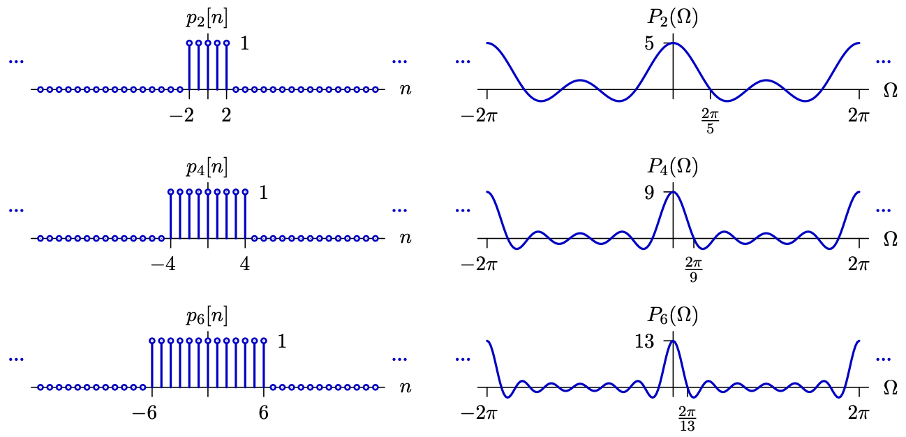
Here's what the Fourier transforms of the $f[n]$ signal from the previous example look like for different values of $S$ .

Because we're working with DT signals, it's hard to formally put into words the time-scaling property.

Other than time-scaling and duality, all of the other CT Fourier transform properties can be ported over to DT easily. (Proofs are obvious.)

Theorem. (Even / Odd) If $f[n]$ is real and even, $F(\Omega)$ is real and even. If $f[n]$ is real and odd, $F(\Omega)$ is imaginary and odd.

Theorem. (Hermitian Symmetry) If $f[n]$ is real, then $F(-\Omega) = \overline{F(\Omega)}$ for all $\Omega$ .

Theorem. (DT Areas) The value of $f[0]$ is $\frac{1}{2\pi} \int_0^{2\pi} F(\Omega) \, \mathrm{d}\Omega$ , and the value of $F(0)$ is $\sum_{n = -\infty}^{\infty} f[n]$ .

Theorem. (Time Delay) The FT of $f[n - n_0]$ is $e^{-j \Omega n_0} F(\Omega)$ .

Theorem. (Derivative FT) If the FT of $f[n]$ is $F(\Omega)$ , then the FT of $g[n] := n f[n]$ is $G(\Omega) = j F'(\Omega)$ .

Theorem. (Kronecker Delta FT) Let the Kronecker delta function $\delta[n]$ be defined so that $\delta[0] = 1$ and $\delta[k] = 0$ for all $k \neq 0$ . The FT of $\delta[n]$ is the constant function $F(\Omega) = 1$ .

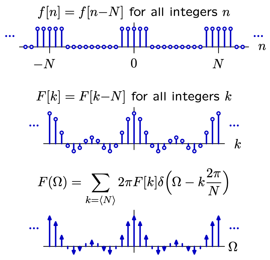
Theorem. (Periodic DT) Suppose $f[n]$ is a periodic signal with Fourier coefficients $F[k]$ , so that $f[n] = \sum_{k = 0}^{N - 1} F[k] e^{jn(2\pi k/N)}$ . Then, treating $F[k]$ as an infinite array with period $N$ , the Fourier transform of $f[n]$ is $F(\Omega) = \sum_{k = -\infty}^{\infty} 2\pi F[k] \delta\left(\Omega - \frac{2\pi k}{N}\right)$ .

Here's what that last theorem looks like visually.