MIT 6.300 — Lecture 13

Discrete Fourier Transform II

§ Lecture: Frequency Resolution

Recall from the end of the Lecture 12 notes what DT and DFT samples tell us about the original CT signal.

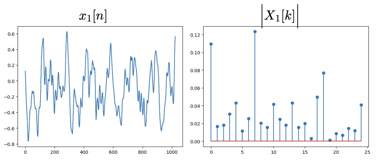
Problem. At a sampling rate of $f_s = 44 \, 100$ , a total of $N = 1024$ samples are taken from a CT signal of a cello, yielding the DT signal $x[n]$ . The DFT of $x[n]$ is $X[k]$ , pictured below.

A zoomed-in graph of $|X[k]|$ for $k \in \{0, 1, \dots, 24\}$ is shown above. Estimate the frequency of the original cello CT signal.

Solution: Note that $\argmax_k |X[k]| = 7$ . The index $k = 7$ in the DFT $X[k]$ corresponds to the frequency $7 \times \frac{f_s}{N} \approx 301.46$ Hz.

More precisely, the true peak frequency must correspond to some index $k \in [6.5, 7.5]$ . This gives us the interval $[280 \, \mathrm{Hz}, 323 \, \mathrm{Hz}]$ , corresponding to frequencies between D4 and Eb4.

Greater values of $N$ will yield a finer frequency resolution. Let's consider one way we might increase the value of $N$ .

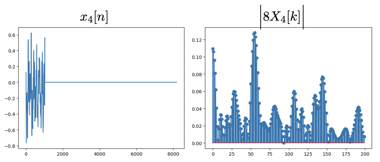
Problem. Let's increase $N$ by a factor of $8$ by defining a new signal $y[n]$ via zero-padding.

y[n] := \begin{cases} x[n] & \text{ if } n \in \{0, 1, \dots, N - 1\}. \\ 0 & \text{ if } n \in \{N, N + 1, \dots, 8N - 1\}. \end{cases}

We then read from $8 \cdot Y[k]$ , where $Y[k]$ is the DFT of $y[n]$ . What frequency data should we expect to obtain from this?

Solution: Recall from Lecture 12 that $Y[k]$ is the result of taking $8 \cdot N$ samples from the DTFT of $y_w[n]$ and dividing them by $8 \cdot N$ . Here's the key:

Claim. The DTFT of $y_w[n]$ is identical to the DTFT of $x_w[n]$ .
$\text{Proof:} ~~~ Y_w(\Omega) = \sum_{n = 0}^{8N - 1} y[n] e^{-j\Omega n} = \sum_{n = 0}^{N - 1} x[n] e^{-j\Omega n} = X_w(\Omega). ~~~ \square$

Thus $8 \cdot Y[k]$ is just a more finely-discretized sampling of $\frac{1}{N} X_w(\Omega)$ than $X[k]$ .

Note that $\argmax_k |8 \cdot Y[k]| = 55$ , which suggests a tighter interval of frequencies $[293 \, \mathrm{Hz}, 298.77 \, \mathrm{Hz}]$ from $k \in [54.5, 55.5]$ . But it would be misleading to be so tight: the peak at $k = 55$ is not very much higher than the peak at, say, $k = 54$ or $k = 56$ .

Through zero-padding, larger values of $N$ will give us a clearer view of the DTFT $X_w(\Omega)$ . But if the DTFT $X_w(\Omega)$ itself is too fuzzy, we still won't get a clearer vision of the correct CT frequency.

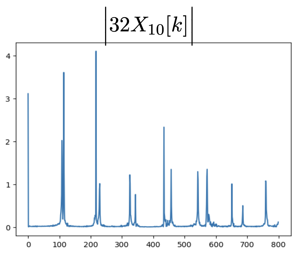
If we want to genuinely increase our frequency resolution, we just need to sample more data. Increasing the length of our DT signal by $\times 32$ to $N = 32 \, 768$ , we arrive at the following.

Only now can we see the truth:

There are actually two frequencies: both D and E-flat! (In addition to their harmonic series…)
The fundamental frequency is an octave lower than expected, at $k = 108$ (or $145 \, \mathrm{Hz}$ ) and $k = 114$ (or $153 \, \mathrm{Hz}$ ).

Zero-padding can make our understanding of the data more precise, but it can't make the data we got any more informative.

§ Lecture and Recitation: Circular Convolution

Definition. Given two arrays $A$ and $B$ and a positive integer $N$ , their circular convolution is:

(A \circledast B)[n] := \sum_{m = 0}^{N - 1} A[m]B[(n - m) \% N].

Remark. It's just polynomial multiplication in the ring $\mathbb{C}[z]/(z^N - 1)$ .

Just as the DTFT of a convolution is the product of the DTFTs, the DFT of a circular convolution is the product of the DFTs.

Theorem. (Circular Convolution = Multiplication) Suppose the DFT of $a[n]$ is $A[k]$ , and the DFT of $b[n]$ is $B[k]$ , both using the same window size $N$ . Then the DFT of $(a \circledast b)[n]$ is $N \cdot A[k] \cdot B[k]$ , and the DFT of $a[n] \cdot b[n]$ is $(A \circledast B)[k]$ .

Proof: Just the same sort of argument as we saw in Lecture 10. For the first direction,

\mathrm{DFT}(a \circledast b)[k] = \frac{1}{N} \sum_{n = 0}^{N - 1} (a \circledast b)[n] e^{-j (2\pi k / N) n} = \frac{1}{N} \underbrace{\left(\sum_{n = 0}^{N - 1} a[n] e^{-j (2\pi k / N)n}\right)}_{ = \ N \cdot A[k] } \underbrace{\left(\sum_{n = 0}^{N - 1} b[n] e^{-j (2\pi k / N)n}\right)}_{ = \ N \cdot B[k] } = N \cdot A[k] \cdot B[k].

It's just polynomial multiplication in the ring $\mathbb{C}[z]/(z^N - 1)$ . And for the inverse direction,

\mathrm{DFT}^{-1}(A \circledast B)[n] = \sum_{k = 0}^{N - 1} (A \circledast B)[k] e^{j (2\pi k / N) n} = \underbrace{\left(\sum_{k = 0}^{N - 1} A[k] e^{j (2\pi k / N)n}\right)}_{ = \ a[n] } \underbrace{\left(\sum_{k = 0}^{N - 1} B[k] e^{j (2\pi k / N)n}\right)}_{ = \ b[n] } = a[n] \cdot b[n].

And that's it; nothing new. $\blacksquare$

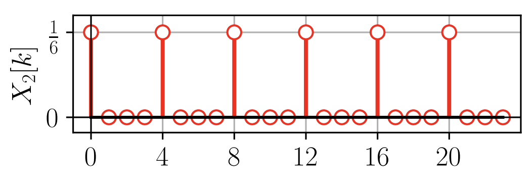
Problem. Consider a DT signal $x[n]$ of length $11$ whose DFT for $N = 16$ (found via zero-padding) is $X[k]$ . Determine how the length- $11$ circular convolution $(x \circledast x)[n]$ relates to the signal $x'[n] := 16 \cdot \mathrm{DFT}^{-1}(X^2[k])$ .

Solution: By the theorem above, we should expect:

x'[n] = \sum_{m = 0}^{10} x[m] x[(n - m)\%16] ~~~ \text{ and } ~~~ (x \circledast x)[n] = \sum_{m = 0}^{10} x[m] x[(n - m)\%11].

So we should expect some time-aliasing errors between $x'[n]$ and $(x \circledast x)[n]$ . For example, suppose $x[n]$ is given by:

x[n] := \begin{cases} 1 & \text{ if } n \in \{1, 2, 4, 8\} \\ 0 & \text{ if } n \in \{0, 3, 5, 6, 7, 9, 10\} \end{cases}.

There is exactly $1$ pair of numbers from $\{1, 2, 4, 8\}$ whose sum is $0$ modulo $16$ —the pair $(8, 8)$ —so $x'[0] = 1$ . However, there is no pair of numbers from $\{1, 2, 4, 8\}$ whose sum is $0$ modulo $11$ , so $(x \circledast x)[0] = 0$ .

§ Recitation: Impulse Trains

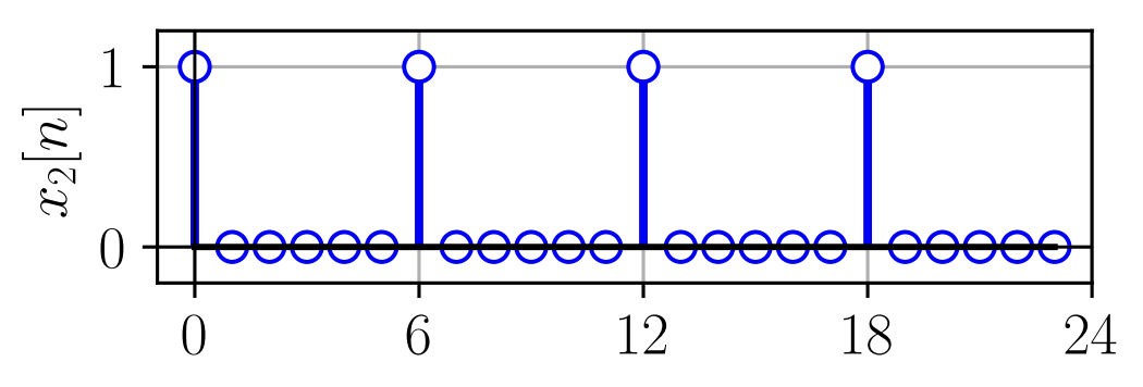
An impulse train is a special kind of periodic signal consisting of repeating evenly-spaced impulses.

An example of an impulse train and its DFT is shown above.

Theorem. (Impulse Trains) The Fourier transform of an impulse train is another impulse train.

Given $f[n] := \sum_{m = -\infty}^{\infty} \delta[n - mN]$ , its DTFT is $F(\Omega) = \frac{2\pi}{N} \sum_{k = 0}^{N - 1} \delta\left(\Omega - k \cdot \frac{2\pi}{N}\right)$ .
Given $f(t) := \sum_{m = -\infty}^{\infty} \delta(t - mT)$ , its CTFT is $F(\omega) = \frac{2\pi}{T} \sum_{k = -\infty}^{\infty} \delta\left(\omega - k \cdot \frac{2\pi}{T}\right)$ .
Given $f[n] := \sum_{m = 0}^{(N / L) - 1} \delta[n - mL]$ where $L \mid N$ , its DFT for window size $N$ is $F[k] = \frac{1}{L} \sum_{m = 0}^{L - 1} \delta\left[k - m \cdot \frac{N}{L}\right]$ .

Proof: Just plain computation. Work it out in your head; the discussion from Lecture 6 on impulses is relevant here. $\blacksquare$