MIT 6.300 — Lecture 15

Short-Time Fourier Transform

§ Lecture: Updated DFT Conventions

This note is purely definitional, but it's an important use of jargon that will be assumed for this lecture.

Definition. Let $x[n]$ be a DT signal with length $s$ . The $\underline{\text{``DFT of size }N\text{''}}$ of $x[n]$ when $N \geq s$ is the result of first zero-padding $x[n]$ to have length $N$ , then taking the length- $N$ DFT of the result.

So far, we've only talked about the $N = s$ case. This lecture will use the $N > s$ case.

Remark. In contrast, the $N < s$ case is completely nonsensical.

§ Lecture: Spectrograms

If you were to shove a recording of a piano playing a single chord through the DFT, you'd be able to retrieve the frequencies of that chord. But if you were to shove a recording of a piano playing an entire song through the DFT, you'd only retrieve the set of all frequencies present in the entire song—not the timing of each frequency, or even what order they came in.

The DFT no longer works when frequencies change over time. If we want to analyze the frequencies in an entire song, we need data that shows the frequencies present at each moment in time.

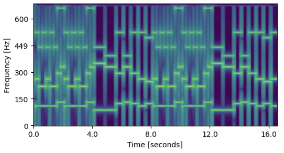
Such data is called a spectrogram, pictured above. It is produced by performing several short-time DFTs.

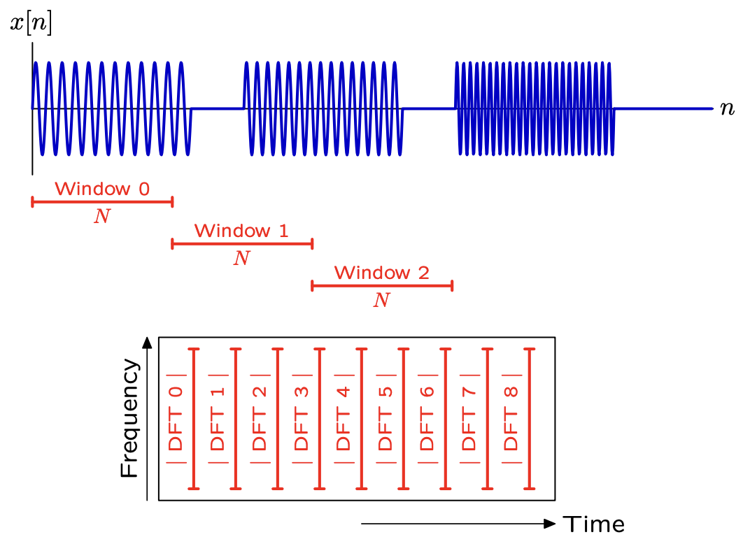
Problem. You're given a DT signal with sampling rate $f_s = 44100$ samples per second and want a spectrogram such that:

Sixteenth notes at a tempo of $120$ beats per minute (each lasting $\frac{1}{8}$ of a second) are distinguished from each other.
Errors in frequency are less than or equal to $5$ Hz.

Determine the range of all possible window lengths $N$ you might use.

Solution: The first condition implies $\frac{N}{f_s} \leq \frac{1}{8}$ , and the second condition implies $\frac{f_s}{N} \leq 10$ . Together, this implies $N \in [4410, 5512]$ .

This process of taking DFTs over sliding windows is known as the Short-Time Fourier Transform (STFT).

§ Lecture: Streaming Windows

Recall from Lecture 10 that applying a band-pass filter to a DT signal $x[n]$ is equivalent to multiplying its DTFT $X(\Omega)$ by a box-shaped frequency response $H(\Omega)$ , which is itself equivalent to convolving $x[n]$ with the unit-sample response $h[n]$ .

In the following discussion, we'll try to isolate the melody of the following.

When working with finite-length DFTs, two issues arise.

The FFT runs in $O(N \log N)$ time. For very long DT signals $x[n]$ , it is not feasible to filter the entire signal at once.
Filtering DT signals via circular convolution gives rise to time aliasing (see Lecture 13), yielding buggy noises.

A natural fix for the first issue is to apply STFT:

Bad Approach. Break $x[n]$ into subsignals $x_i[n]$ of length $N$ . For each subsignal, compute $x_i'[n] := (x_i \circledast h)[n]$ , where $h[n]$ is a length- $N$ unit-sample response of a band-pass filter. Finally, concatenate all of the $x_i'[n]$ together. Here's how the result sounds:

Clearly something sounds off. The main issue comes from our neglect of issue #2: circular convolution and time-aliasing.

Remark. The reason why circular convolution fails is subtle. It is true that each $x_i'[n]$ only contains frequencies inside the desired band. But consider the following two extensions of $x_i'[n]$ from the domain $[0, N - 1]$ to the domain $\mathbb{N}$ .

x_i'^{\,(1)}[n] := x_i'[n \% N] ~~~ \text{ and } ~~~ x_i'^{\,(2)}[n] := \begin{cases} x_i'[n] & \text{ if } n \in [0, N - 1]. \\ 0 & \text{ otherwise.} \end{cases}

All that can be said is that the DTFT of $x_i'^{\,(1)}[n]$ contains only band frequencies—but not for $x_i'^{\,(2)}[n]$ . Yet the concatenation of all of the $x_i'[n]$ is the sum of the $x_i'^{\,(2)}[n]$ —not the $x_i'^{\,(1)}[n]$ .

Therefore, there is no reason for the DTFT of the concatenation of the $x_i'[n]$ to only contain band frequencies.

We really should be taking a linear convolution, not a circular convolution, meaning we need to allow time in one window to overflow into the next, rather than aliasing it back around.

Good Approach (Overlap-Add — Time Domain). Break $x[n]$ into subsignals $x_i[n]$ of length $s$ . For each subsignal, compute the length- $N$ subsignal $x_i'[n] := (x_i * h)[n]$ , where $h[n]$ is a length- $(N - s + 1)$ unit-sample response of a band-pass filter.

Finally, add all of the $x_i'[n]$ together.

Note that each window's linear convolution overlaps with the linear convolutions from other windows—hence the name “overlap-add” and not “overlap-concatenate”.

We can equivalently think of overlap-add from the frequency domain.

Good Approach (Overlap-Add — Frequency Domain). Break $x[n]$ into subsignals $x_i[n]$ of length $s$ . For each subsignal, zero-pad $x_i[n]$ to have length $N$ , then compute its DFT $X_i[k]$ of size $N$ . Then compute the element-wise products $X_i'[k] := N \cdot X_i[k] \cdot H[k]$ , where $H[k]$ is a length- $N$ frequency response of a band-pass filter.

Finally, compute the length- $N$ subsignals $x_i' := \mathrm{DFT}^{-1}(X_i')$ and sum them together.

Note that $H[k]$ is the DFT of size $N$ of $h[n]$ , where the length of $h[n]$ is only $N - s + 1$ . (Implicitly, we zero-pad $h[n]$ first…)

There are two reasons for wanting to think from the perspective of the frequency domain.

It's how we would go about algorithmically implementing such a filter.
- Naive linear convolution is $O(N^2)$ , but two DFTs plus an element-wise product is $O(N \log N)$ .
It lets us think more closely about filter design: a better filter will have a better $H[k]$ .

We'll discuss that second point in the next section: designing $H[k]$ and $h[n]$ .

§ Lecture: Short-Time Filter Design

The challenge is that $H[k] = \mathrm{DFT}(h[n])$ , yet $h[n]$ has some length $N_f = N - s + 1$ that is less than the length of $H[k]$ . We must compromise in our design of $H[k]$ so that the last $N - N_f$ entries of $\mathrm{DFT}^{-1}(H[k])$ are all zeroes.

Box Approach. Let's work in reverse: we'll design an $h[n]$ of length $N_f$ , then hope the $H[k]$ we get is an effective filter.

Take a perfect (continuous) filtering frequency response $H_1(\Omega)$ . No compromises here.

Define $h_1[n]$ to be the discretized version of the impulse response $\mathrm{DTFT}^{-1}(H_1(\Omega))$ , truncated to length $N_f$ .

Define $h_2[n]$ to be a version of $h_1[n]$ that is zero-padded to have length $N$ .

Define $H_2[k] := \mathrm{DFT}(h_2[n])$ of length $N$ .

Then $H_2[k]$ is our designed frequency response $H[k]$ . Here's how the result sounds when used with overlap-add:

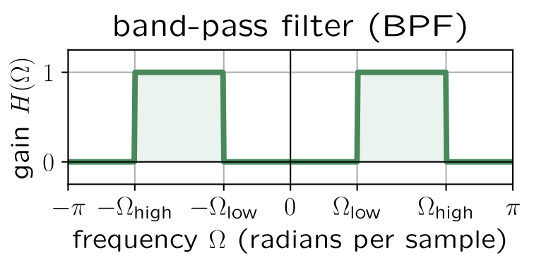
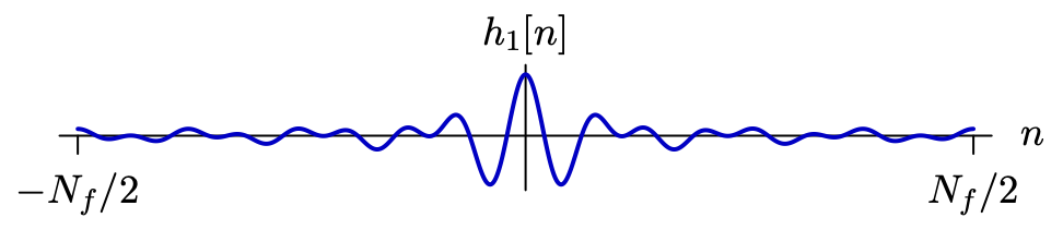
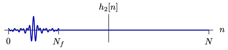
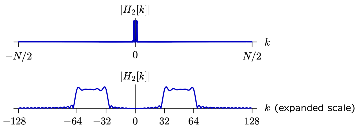
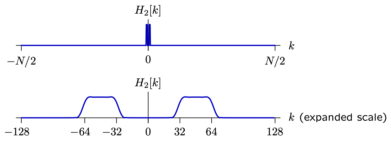
That works pretty well! But if you listen closely, you can still faintly hear some of the frequencies from the harmony, especially in the second half. You can see why in the graph of $H_2[k]$ : the graph has “ripples” that make it an imperfect filter.

These ripples come from Step #2: ideally, we would take $h_1[n] := \mathrm{DTFT}^{-1}(H_1(\Omega))$ to be an infinite DT signal, but instead, we must compromise by truncating to have length $N_f$ .

Here's the trick, though: what if we truncated a bit more smoothly?

Hann Window Approach. We take the same approach as before, but we instead define $h_1[n]$ as follows.
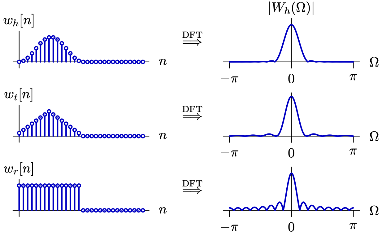
$h_1[n] := w_h[n] \cdot \mathrm{DTFT}^{-1}(H_1(\Omega)) ~~~ \text{ where } ~~~ w_h[n] := \begin{cases} \sin\left(\frac{\pi n}{N_f}\right)^2 & \text{ if } n \in [0, N_f - 1] \\ 0 & \text{ otherwise.} \end{cases}$
The signal $w_h[n]$ is called a Hann Window, in contrast to the typical rectangular window
$w_r[n] := \begin{cases} 1 & \text{ if } n \in [0, N_f - 1] \\ 0 & \text{ otherwise.} \end{cases}$
used in the previous approach. Yet another alternative choice is a triangle window; you can observe the efficacy of each of these truncation methods through the diagram below.

In the previous approach, the frequencies present in $h_1[n]$ would be the result of convolving our perfect filter $H_1(\Omega)$ with the ripple-filled signal $\mathrm{DTFT}(w_r[n])$ . No wonder the result $H_2[k]$ had so many ripples!

Expectedly, using the Hann window to construct the truncation $h_1[n]$ gives a much cleaner $H_2[k]$ .

And it sounds much better, too—no more harmonies still lingering around.

§ Recitation: Windows and Decibels

We already saw how the rectangular, triangular, and Hann windows compare. But let's compare them at a logarithmic scale.

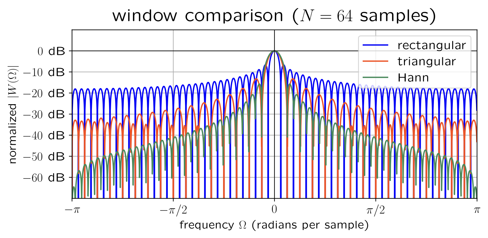
In the above, decibels are a relative unit of measurement. (So turning the volume knob up won't alter these graphs.)

Definition. Given a signal $x[n]$ , say its highest value is $M$ . Then $x[n]$ in decibels is $10 \log_{10}\left(\frac{x[n]}{M}\right)$ .

So a measurement of $-20$ dB corresponds to a measurement in the signal that is $\times \frac{1}{100}$ the highest measurement. For reference, measurements of $-60$ dB are essentially inaudible, whereas measurements of $\approx -25$ dB are still weakly perceptible.

§ Recitation: Short-Time Fourier Transform

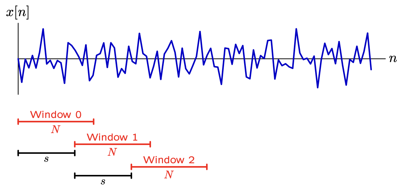
We never actually formally defined the STFT. Let's do that.

Definition. Given a signal $x[n]$ and a window $w[n]$ , the STFT is the two-dimensional array:

X[k, m] := \frac{1}{N} \sum_{n = 0}^{N - 1} x[n + ms] \cdot w[n] \cdot e^{-jk \frac{2\pi}{N} n}.

Note that $k$ and $m$ each only appear once on the RHS. The value of $k$ controls the frequency being measured, and the value of $m$ controls the time being measured. A spectrogram is a diagram that displays $|X[k, m]|^2$ .

Note that the STFT of $x[n]$ depends on three different parameters:

w[n]: \text{ the type of window } ~~~ \parallel ~~~ N: \text{ the DFT size } ~~~ \parallel ~~~ s: \text{ the step size }

Importantly, $\mathrm{len}(w[n])$ , $N$ , and $s$ do not have to be equal!

You can take $s < \mathrm{len}(w[n])$ , meaning each data point will be used multiple times!
- Or $s > \mathrm{len}(w[n])$ , meaning some data points are completely ignored…
You can take $N > \mathrm{len}(w[n])$ , meaning the data collected from the window $w[n]$ will be zero-padded to have length $N$ .
- It does not make sense to take $N < \mathrm{len}(w[n])$ . You cannot take a DFT of size $6$ on a DT signal of length $7$ .

Compare the cleanliness of a rectangular window (at left) versus a Hann window (at right).

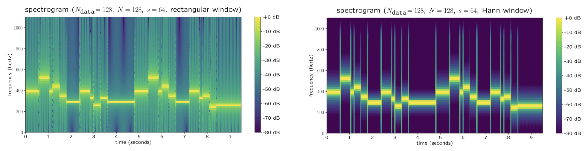
Expectedly, the parameter settings affect the spectrogram as follows.

Increasing $\mathrm{len}(w[n])$ increases the frequency resolution, at the cost of time resolution.
Increasing $N$ increases the fineness of frequency measurements—but only superficially. (Recall Lecture 13.)
Decreasing $s$ increases the fineness of time measurements.

Of course, these improvements to parameter settings come at a cost of time complexity.