MIT 6.300 — Lecture 2

Sinusoids and Series

§ Lecture: Convergence

Here is the graph of the Fourier series of a square wave, truncated to its first hundred terms.

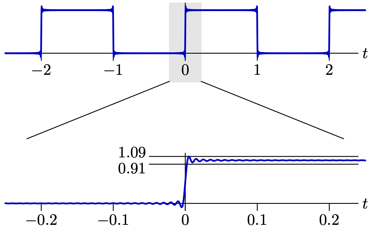
Notice how the discontinuity of the square wave presents itself in its Fourier series. It turns out that the $9\%$ error shown above never goes away, even as arbitrarily many terms are added!

Theorem. (Gibbs' Phenomenon) Suppose a (sufficiently well-behaved) signal $f(t)$ has a “step discontinuity” at $t = t_0$ ; that is,

L = \lim_{t \to t_0^-} f(t) \neq \lim_{t \to t_0^+} f(t) = R.

Furthermore, let $f_K(t)$ denote the partial sum of the first $K$ terms of the Fourier series for $f(t)$ . Then the following hold:

Evaluated at $t = t_0$ , the Fourier series converges to $\frac{1}{2}(L+R)$ .
Near $t_0$ , the partial sum $f_K$ overshoots $R$ and undershoots $L$ by an amount converging to $\approx 9\% \cdot (R - L)$ (assuming $R > L$ ).
For any $\epsilon > 0$ , the length of the interval over which $|f(t) - f_K(t)| > \epsilon$ shrinks to zero as $K \to \infty$ .

In particular, the Fourier series of a discontinuous function converges pointwise, but not uniformly.

The exact value of the $9\%$ constant is $\dfrac{1}{\pi} \displaystyle \int_0^\pi \dfrac{\sin(t)}{t} \, \mathrm{d}t - \dfrac{1}{2} \approx 0.08949$ .

§ Lecture: Transforming Fourier Series

Problem. Given the Fourier coefficients $(c_0, c_k, d_k)$ for $f(t)$ , determine the Fourier coefficients of $f(2t)$ .

Solution: The only difference between $f(2t)$ and $f(t)$ is in their fundamental frequencies. The Fourier coefficients do not change.

Remark. Think of the Fourier coefficients as describing the quality of a signal. A piano and a trumpet playing 440 Hz will have different qualities, but a piano playing 440 Hz and a piano playing 880 Hz will not (assuming ideal conditions).

Problem. Given the Fourier coefficients $(c_0, c_k, d_k)$ of $f(t)$ , determine the Fourier coefficients of $f(t - T/2)$ .

Solution: Just note the following (recalling that $\omega_0 = \frac{2\pi}{T}$ always):

\cos\left(k \omega_0 \left(t - T/2\right)\right) = (-1)^k \cos(k \omega_0 t) ~~~ \parallel ~~~ \sin\left(k \omega_0 \left(t - T/2\right)\right) = (-1)^k \sin(k \omega_0 t).

Thus, odd-indexed coefficients are negated, and all other coefficients remain unchanged.

§ Recitation: Symmetry in Fourier Series

Recall from Lecture 1 that it's easy to compute the Fourier series of an even or odd function.

Theorem. (Everything is Even/Odd) Every function $f(t)$ can be expressed as the sum of an even function and an odd function.

f(t) = \underbrace{\left(\dfrac{f(t) + f(-t)}{2}\right)}_{\text{even}} + \underbrace{\left(\dfrac{f(t) - f(-t)}{2}\right)}_{\text{odd}}

Proof: The proof is in the statement of the theorem itself. $\blacksquare$

In 6.300, “symmetric” and “antisymmetric” mean “even” and “odd”, respectively—and “asymmetric” means neither.

Thus, if an asymmetric signal can be easily expressed as the sum of a symmetric and antisymmetric signal, then computing its Fourier series might be easier to do in two steps…