MIT 6.300 — Lecture 4

Sampling, Aliasing, and DT Signals

§ Lecture: Sampling and Aliasing

In practice, we might have to settle for discretized samples of data, rather than the full continuous signal.

Definition. Let $\Delta$ be our sampling interval and $f_s = \frac{1}{\Delta}$ be our sampling frequency. Our data is then the discrete-time (DT) signal $x[n] = f(\Delta n)$ , as opposed to the continuous-time (CT) signal $f(t)$ .

Remark. Just as CT signals have a fundamental period, so too can DT signals—but their fundamental periods must be integers! (And as we'll see later, some DT signals have no fundamental period at all.)

But an insufficiently fine sampling might yield misleading results!

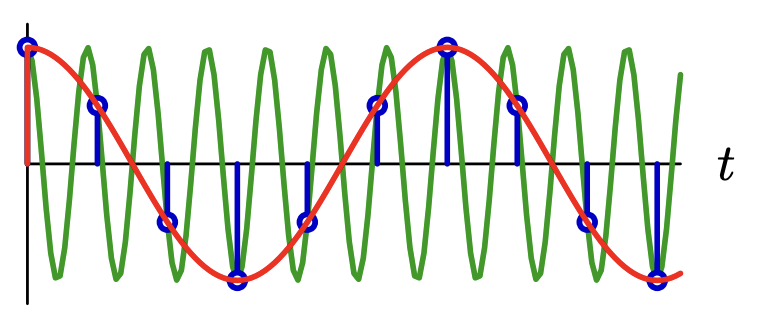
Definition. If signals $f_1(t) = \cos(\omega_1t)$ and $f_2(t) = \cos(\omega_2t)$ generate the same discrete samples, we say $\omega_1$ and $\omega_2$ are aliases.

Remark. We only consider pure cosine signals because it turns out they result in the most possible aliasing.

So in the picture above, the frequencies of the red and green curves are aliases.

Theorem. (Aliasing Classification) Frequencies $\omega_1$ and $\omega_2$ are aliases if and only if $\omega_2 \Delta = 2\pi k \pm \omega_1 \Delta$ for some $k \in \mathbb{Z}$ .

Proof: Aliasing occurs if and only if we have $\cos(\omega_1 \Delta n) = \cos(\omega_2 \Delta n)$ for all $n \in \mathbb{Z}$ . Note the following:

\cos(\omega_1 \Delta n) - \cos (\omega_2 \Delta n) = -2 \sin\left(\frac{\omega_1 \Delta + \omega_2 \Delta}{2} \cdot n\right) \sin\left(\frac{\omega_1 \Delta - \omega_2 \Delta}{2} \cdot n\right).

The above is always zero if and only if either $\omega_1 \Delta + \omega_2 \Delta$ or $\omega_1 \Delta - \omega_2 \Delta$ is an integer multiple of $2\pi$ . $\blacksquare$

One anti-aliasing tactic is to assume that all frequencies are below the Nyquist frequency $\omega_m := \frac{\pi}{\Delta}$ . This way, as long as $\omega_1$ and $\omega_2$ are assumed to be below $\omega_m$ , it is impossible for them to be aliases unless they are equal.

Equivalently, every frequency $\omega$ has a unique baseband frequency $\omega' \leq \omega_m$ such that $\omega$ and $\omega'$ are aliases.

Problem. Determine the baseband frequency of $f(t) = \cos(4000 t)$ when $\Delta = 0.001$ .

Solution: The frequency is $\omega = 4000$ , which gives $\omega \Delta = 4$ . In order to be a valid baseband frequency $\omega'$ , we require $\omega' \Delta \leq \pi$ . Thus, we take the alias $\omega'$ such that $\omega' \Delta = 2\pi - \omega \Delta = 2\pi - 4$ , yielding a baseband frequency of $\omega' = 2000\pi - 4000$ .

Remark. Check your intuition: when $\Delta$ is smaller, the baseband frequency is more likely to match the original frequency.

§ Lecture: Quantization

Another way we can discretize data is by restricting the number of bits used to represent each individual sample.

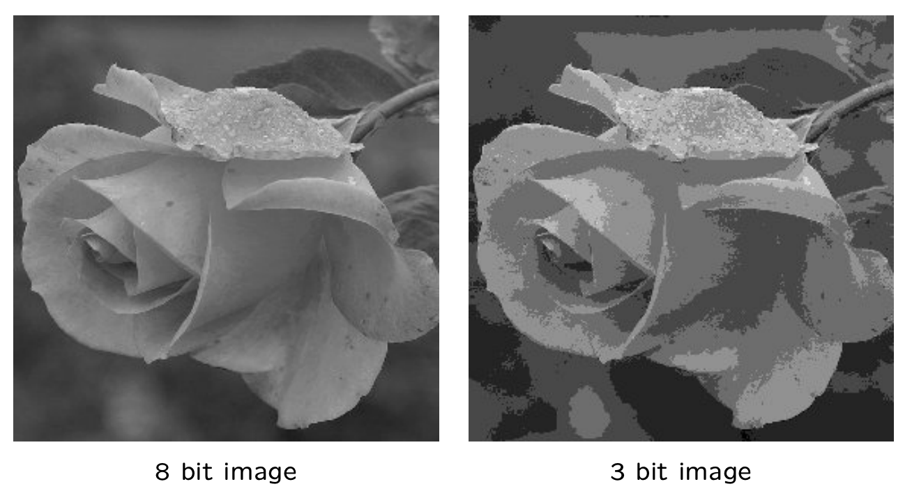
(We'll never bring this up in 6.300 ever again.)

§ Recitation: The Sampling Theorem

Here's what it looks like to take more than 2, exactly 2, and fewer than 2 samples per cycle.

We can observe the following:

When we sample more than 2 times, the samples represent the frequency pretty well.
When we sample exactly 2 times, the samples still capture the frequency—but practically nothing else.
When we sample fewer than 2 times, the samples capture the wrong frequency—it appears to be $\frac{2}{3}$ of the original.

In a sense, it takes at least 2 samples per cycle to preserve the information in a sinusoid.

Theorem. (Sampling Theorem) If $f_{\text{max}}$ is the highest nonzero (cyclical) frequency in a CT signal, then a sampling rate $f_s > 2 f_{\text{max}}$ is enough to prevent all aliasing.

Remark. Here's a trick question.

Question. Humans cannot hear frequencies above 20 kHz. Does this mean a sampling rate of 40 kHz suffices?

The answer is no. None of the frequencies we can hear will alias, but frequencies above 20 kHz that we can't hear will alias into frequencies that we can hear, thus distorting the recording.

§ Recitation: Dimensional Analysis

We've been using the word “frequency” pretty carelessly so far. But the introduction of $\Delta$ and $f_s$ complicates things.

Definition. The CT signal $f(t) = \sin(K t)$ has an angular frequency of $\omega_0 := K$ and a cyclical frequency of $f_0 := \frac{K}{2\pi}$ . Angular frequency has units radians per second, and cyclical frequency cycles per second (or Hz).

Definition. The DT signal $f[n] = \sin(K n)$ has an angular frequency of $K$ and a cyclical frequency of $\frac{K}{2\pi}$ . Angular frequency has units radians per sample (dimensionless!), and cyclical frequency cycles per sample (dimensionless!).

Remark. The cyclical frequency of a CT signal is measured in Hz, but the cyclical frequency of a DT signal is technically not!

Cyclical frequency has become relevant with the introduction of $f_s = \frac{1}{\Delta}$ , the sampling frequency (in samples per second).

Problem. A pure-sine $5\pi$ Hz CT signal is sampled at an interval of $\Delta = \pi^2$ . Determine the resulting DT signal.

Solution: A pure-sine $5\pi$ Hz CT signal looks like $f(t) = \sin(10\pi^2 t)$ . The DT signal then looks like $f[n] = \sin(10 \pi^4 n)$ .

We can then read off the following.

The angular frequency is $10\pi^4$ radians per sample.
- But radians are a measurement taken modulo $2\pi$ . We could also say the angular frequency is $10\pi^4 \pmod{2\pi} \approx 0.19719$ .
The cyclical frequency is $\frac{10\pi^4}{2\pi} = 5\pi^3$ cycles per sample.
- But cycles are a measurement taken modulo $1$ . We could also say the cyclical frequency is $5\pi^3 - \lfloor 5\pi^3 \rfloor \approx 0.031383$ .

Note, importantly, that it does not make sense to call the fundamental angular frequency $\Omega_0 \approx 0.19719$ , say. This is because this DT signal isn't periodic! It doesn't have a “fundamental frequency” that we can use to (say) write a Fourier series.

Remark. We just say that if a DT signal has an angular frequency of $K$ , then $K' = K \pm 2k \pi$ is also a valid angular frequency for all $k \in \mathbb{Z}$ . However, this does not hold for CT signals: samples are a discrete measurement, but time is not.

(A more mathematical reason why this does not apply for CT signals is that $e^{2\pi j t} \neq 1$ for $t \not \in \mathbb{Z}$ .)

§ Recitation: Periods of DT Signals

As we just saw, sinusoidal CT signals always have a fundamental period, but DT signals might not…

Definition. The CT signal $f(t) = \sin(Kt)$ has a fundamental period $T$ , with the relationship $T = \frac{2\pi}{K}$ .

Definition. The DT signal $f[n] = \sin(Kn)$ has a fundamental period $N$ only if $\frac{2\pi}{K}$ is rational, in which case $N$ is the numerator of $\frac{2\pi}{K}$ in simplest form.

Definition. If a DT signal has fundamental period $N$ , then its fundamental angular frequency is $\Omega_0 := \frac{2\pi}{N}$ , and its fundamental cyclical frequency is $F_0 := \frac{1}{N}$ . (Aperiodic DT signals do not have fundamental angular / cyclical frequencies.)

Warning! For DT signals $f[n] = \sin(Kn)$ , the relationships $\Omega_0 = K$ and $N = \frac{2\pi}{K}$ are not guaranteed!

Remark. Of course, nothing is special about $\sin$ here—all of this applies equally well to $\cos$ too.

Problem. The DT signals $f[n] = \cos(1.2\pi n)$ and $g[n] = \cos(2.8\pi n)$ are the same, and they both have fundamental periods. What do $\Omega_0$ , $F_0$ , $N$ , $\frac{2\pi}{\Omega_0}$ , and $\frac{1}{F_0}$ equal for each of them?

Solution: Both signals are the same, with $N = 5$ , so they have the same results: $(\Omega_0, F_0, N, \frac{2\pi}{\Omega_0}, \frac{1}{F_0}) = (0.4\pi, 0.2, 5, 5, 5)$ .

Checking whether a DT signal even has a fundamental period cannot be easily overlooked!

Problem. Suppose an $f_0$ Hz CT signal is sampled at a sampling rate of $f_s = 44 \, 100$ Hz. What must be true about $f_0$ for the resulting DT signal to have a fundamental period?

Solution: Simply that $f_0 \in \mathbb{Q}^+$ . The fundamental period is the numerator of $\frac{f_s}{f_0}$ . So the fundamental period equals $1$ for $f_0 \in \{44 \, 100, 441 \, 000\}$ , is fairly small for $f_0 \in \{200, 420\}$ , and is fairly large for $f_0 \in \{199, 420.01, 0.0042\}$ .

Let's put this together with the sampling / aliasing discussion from earlier.

Problem. A $220$ Hz CT signal is sampled at a sampling interval of $\Delta = 0.0025$ seconds per sample. Determine $N$ , $\Omega_0$ , and $F_0$ for the resulting DT signal. Is there aliasing? How would the DT signal sound if played back at the same sampling rate?

Solution: Note that we are sampling at a sampling rate of $f_s = 400$ Hz, which is smaller than $2f_0 = 440$ . So the Sampling Theorem suggests there might be some aliasing.

The CT signal is $f(t) = \cos(440\pi t)$ , so the DT signal is $f[n] = \cos\left(\frac{11}{10}\pi n\right)$ . Thus $N = 20$ , so $\Omega_0 = \frac{\pi}{10}$ and $F_0 = \frac{1}{20}$ . If we were to perform a Fourier analysis of this signal (see Lecture 5), the only nonzero coefficients would be the $9^{\text{th}}$ and $11^{\text{th}}$ harmonics.

Of course there is aliasing—there is always aliasing—but here, the original frequency of $\omega_0 = 440\pi$ was above the Nyquist frequency of $\omega_m = 400\pi$ . The baseband frequency is $360\pi$ ; indeed, sampling a $180$ Hz signal yields $f'[n] = \cos\left(\frac{9}{10}\pi n\right) = f[n]$ .

If someone were given only the DT signal, they would have no way of knowing the original signal was $220$ Hz. Assuming the baseband frequency were the original frequency, it would seem like the original signal was $180$ Hz. And that's how it turns out in practice: this poorly-sampled DT signal would sound like $180$ Hz when played back at the original rate!