MIT 6.300 — Lecture 12

Discrete Fourier Transform I

§ Lecture: Discrete Fourier Transform

The problem with Fourier transforms is that, unlike Fourier series, they are not easily expressible in code: they're continuous data, not discrete. The discrete Fourier transform, as its name suggests, is the fix for this.

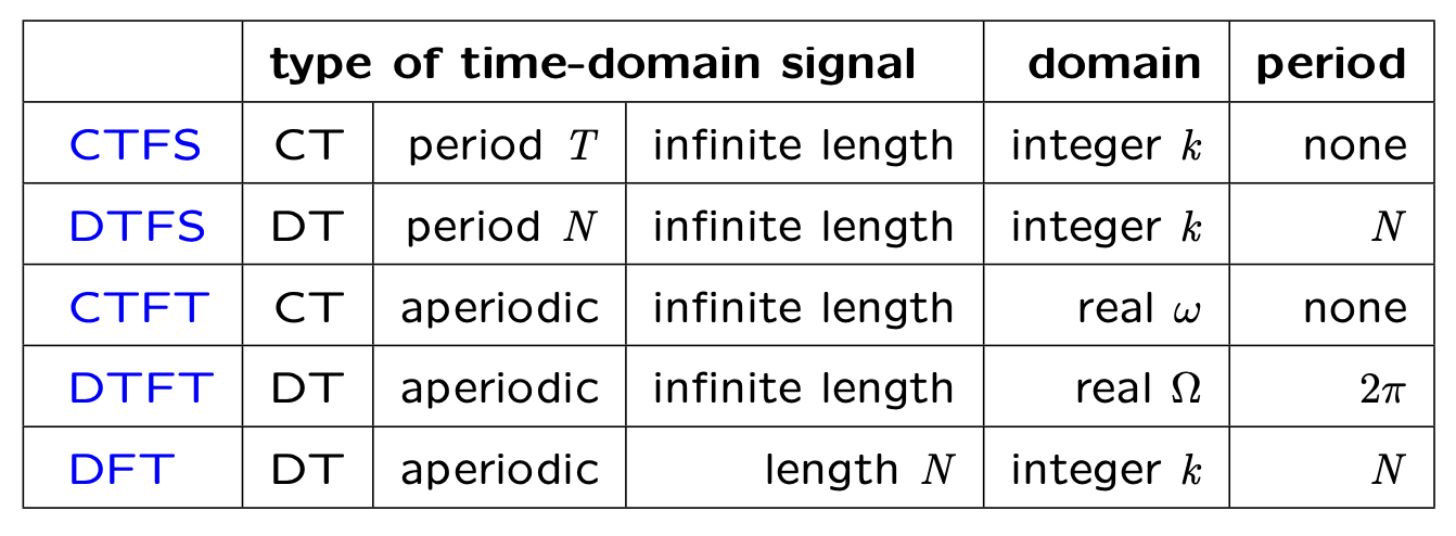
Definition. Given a possibly aperiodic DT signal $x[n]$ and any positive integer $N$ , the discrete Fourier transform (DFT) of $x[n]$ is the same as the Fourier series of the periodic signal $x'[n] := x[n \% N]$ .

Remark. Recall that this means the DFT of $x[n]$ is an array $X$ , where $X[k]$ denotes the coefficient of $e^{j(2\pi k/N)n}$ in the DT Fourier series of $x'[n]$ . Note that $X$ is an array of length $N$ .

Importantly, it does not make sense to ask for “the DFT of $x[n]$ ”. One must always also specify a length $N$ .

In some ways, the DFT is the culmination of all of the Fourier analysis in 6.300 up to this point: it combines the signal-aperiodicity of the DTFT with the computational feasibility of the DTFS.

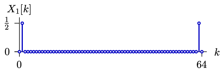
Example. The DFT of $x[n] = \cos\left(\frac{2\pi n}{64}\right)$ for $N = 64$ is the same as the Fourier series of $x[n]$ , plotted below.

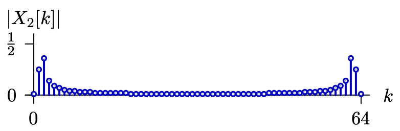
Example. The DFT of $x[n] = \cos\left(\frac{3\pi n}{64}\right)$ for $N = 64$ , plotted below, differs from the Fourier series of $x[n]$ .

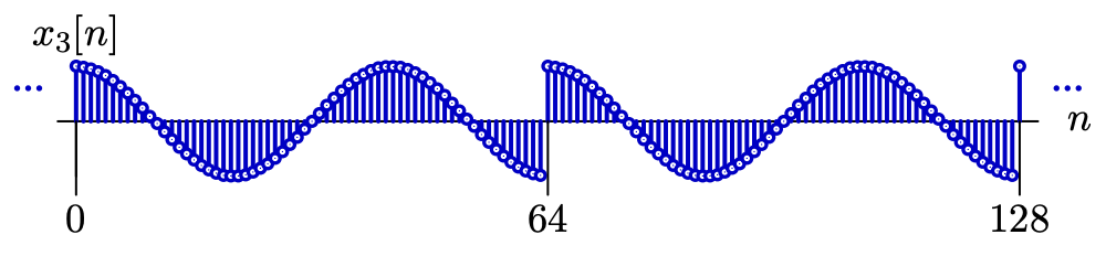
The reason why is that $x[n]$ does not have period $N = 64$ ; its period is $128$ . However, the DFT of $x[n]$ for $N = 64$ does match the Fourier series of the signal pictured below.

Unsurprisingly, here's what the analysis and synthesis equations for the DFT look like.

Theorem. (DFT Formulas) Given a DT signal $x[n]$ and a positive integer $N$ , the DFT of $x[n]$ is $X[k] := \frac{1}{N} \sum_{n = 0}^{N - 1} x[n] e^{-j \frac{2\pi k}{N} n}$ , which satisfies $x[n] = \sum_{k = 0}^{N - 1} X[k] e^{j \frac{2\pi k}{N} n}$ for all $n = 0, 1, \dots, N - 1$ .

These formulas look exactly the same as the DT Fourier series formulas presented in Lecture 5, expectedly.

§ Lecture: DFT vs. DTFT and Windows

We know the relationship between the DFT and the DTFS: they're exactly the same. What about the DFT and the DTFT?

Theorem. (DFT vs. DTFT) Consider a DT signal $x[n]$ and a positive integer $N$ . Define a new signal $x_w[n]$ as follows:

x_w[n] := \begin{cases} x[n] & \text{ if } n \in [0, N - 1]. \\ 0 & \text{ otherwise.} \end{cases}

Suppose $X[k]$ is the DFT of $x[n]$ , and $X_w(\Omega)$ is the DTFT of $x_w[n]$ . Then $X[k] = \frac{1}{N} X_w\left(\frac{2\pi k}{N}\right)$ .

In other words, $X[k]$ is the result of taking $N$ samples from $X_w$ at an interval of $\frac{2\pi}{N}$ and dividing all samples by $N$ .

Proof: Recall from Lecture 7 that the DTFT $X_w(\Omega)$ is defined via $X_w(\Omega) = \sum_{n = -\infty}^{\infty} x_w[n] e^{-j \Omega n}$ . Comparing with the formula $X[k] := \frac{1}{N} \sum_{n = 0}^{N - 1} x[n] e^{-j \frac{2\pi k}{N} n}$ for the DFT, the relationship is immediate. $\blacksquare$

The diagram below paraphrases the statement of the theorem above.

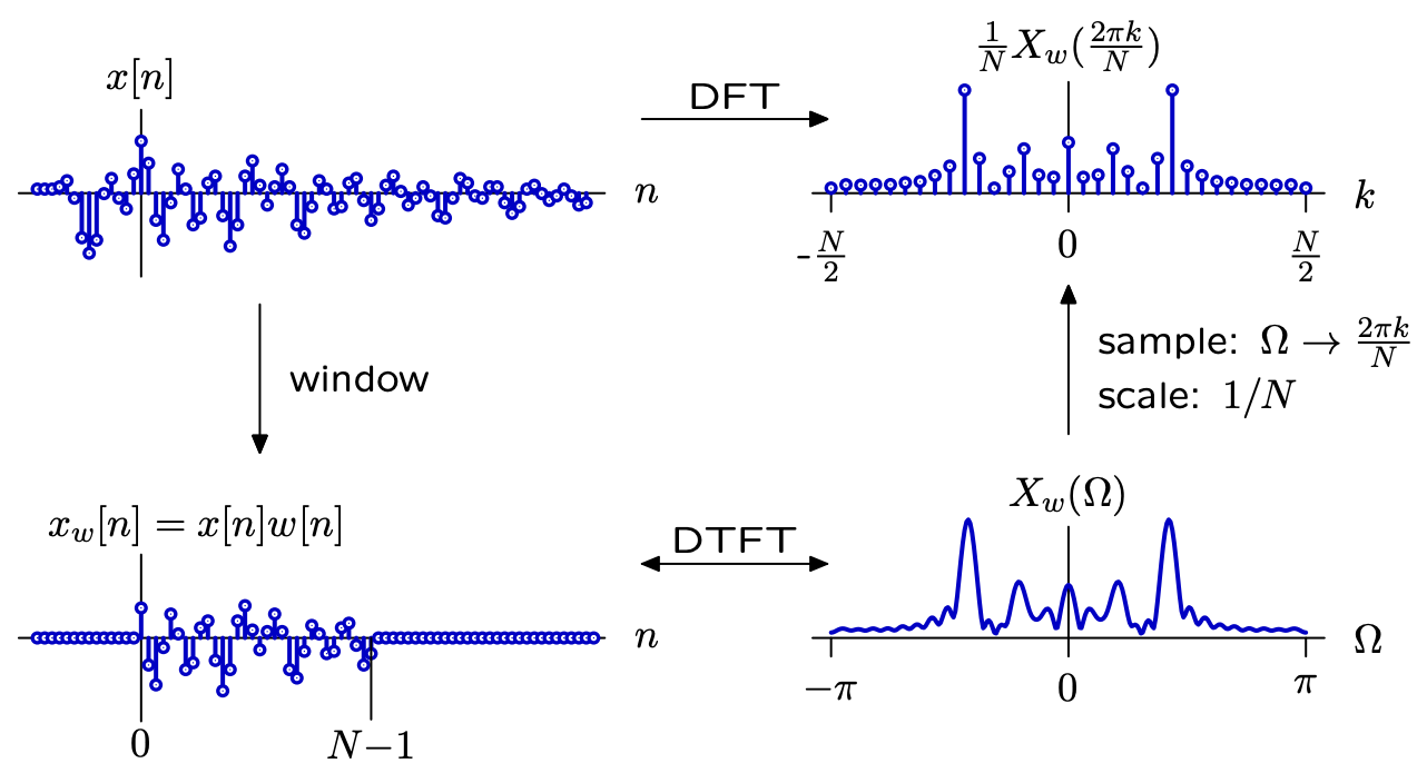
To summarize: the DFT of a DT signal $x[n]$ can be thought of as either…

… the DTFS of a periodic extension $x'[n] := x[n\%N]$ of $x[n]$ , or…
… a scaled, length- $N$ sampling of the DTFT of a windowed version $x_w[n]$ of $x[n]$ , using a window of length $N$ .

Note that the constant $N$ decides the size of the “window” that our DFT takes into account.

Problem. Compute the DFT of the pure-frequency DT signal $x[n] := e^{j\Omega_0 n}$ for varying window sizes $N$ .

Solution: Equivalently, we compute the DTFT of $w[n] \cdot x[n]$ , where $w[n]$ is the signal given by:

w[n] := \begin{cases} 1 & \text{ if } n \in [0, N - 1] \\ 0 & \text{ otherwise.} \end{cases}

Note that the DTFT of $w[n]$ itself looks like the following:

W(\Omega) = \sum_{n = -\infty}^{\infty} w[n] e^{-j \Omega n} = \sum_{n = 0}^{N - 1} e^{-j \Omega n} = \frac{1 - e^{-j \Omega N}}{1 - e^{-j \Omega}} = \left[\frac{ \sin \left(\frac{N \Omega}{2}\right) }{ \sin \left(\frac{\Omega}{2}\right) }\right] \cdot e^{-j \Omega(N - 1) / 2}.

Now we invoke a “dual” of one of the properties from Lecture 7: the DTFT of $w[n] \cdot x[n] = w[n] \cdot e^{j\Omega_0 n}$ is just $W(\Omega - \Omega_0)$ .

Thus, the DFT of $x[n]$ is the result of sampling from $W(\Omega - \Omega_0)$ at intervals of $\frac{2\pi}{N}$ and dividing the samples by $N$ .

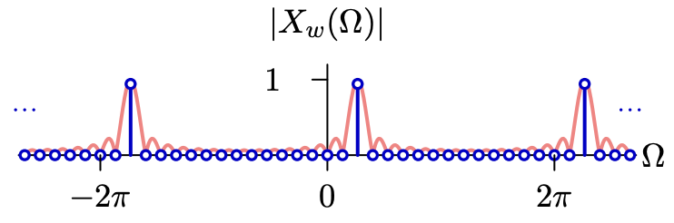
For $N = 15$ and $\Omega_0 = \frac{4\pi}{15}$ (shown above), the resulting DFT reads as strong evidence that the original DT frequency was $\frac{4\pi}{15}$ .

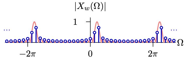
For $\Omega_0 = \frac{3.2\pi}{15}$ (shown above), the resulting DFT is less informative…

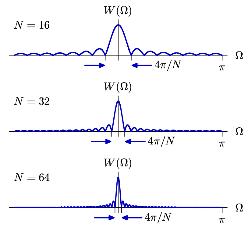
We can get more informative DFTs by increasing the window size $N$ . The larger the value of $N$ , the finer our frequency resolution, and the more samples we get to read.

§ Recitation: Spectral Analysis (Interpreting the DFT)

Problem. A DT signal $x[n]$ is produced by sampling from a CT signal with sampling frequency $f_s$ , and its DFT $X[k]$ is computed using a window length of $N$ . Assume $x[n]$ is periodic modulo $N$ . What does $X[7]$ say about the original CT signal?

Solution: Since $x[n]$ is periodic modulo $N$ , the DFT of $x[n]$ is very informative: it's exactly the same as the DTFS of $x[n]$ .

The rest is dimensional analysis. Note that $X[7]$ is the coefficient of $e^{j(2\pi(7)/N)n}$ in the DTFS, so it represents the strength of the discrete-time angular frequency $\Omega_0 = 7 \times \frac{2\pi}{N}$ .

In continuous-time, this translates to (recalling Lecture 4) a continuous-time angular frequency of $\omega_0 = 7 \times \frac{2\pi}{N} \times f_s$ .

More generally, we can say the following:

Theorem. (Spectral Analysis) The DFT $X[k]$ measures the strength of the continuous-time cyclical frequency $f_0 = \frac{k}{N} \times f_s$ .

Problem. Suppose $f_s = 44 \, 100$ , and consider a DFT $X[k]$ using window size $N = 100$ . Given that $X[13] = X[87] = 1$ and all other entries of $X$ are zero, what can we say about the original CT signal?

Solution: The original CT signal probably had a cyclical frequency of $\frac{13}{100} \times 44 \, 100 = 5 \, 733$ Hz.

Notably, the data provided by the DFT is discrete, so the set of CT frequencies it may tell us about is also discrete.

Definition. Two angular frequencies $\Omega_1$ and $\Omega_2$ are resolved (that is, distinguishable in the DFT) if $|\Omega_1 - \Omega_2| > \Delta\Omega$ , where $\Delta\Omega := \frac{2\pi}{N}$ is the frequency resolution. (For cyclical frequencies, it looks like $\Delta f := \frac{f_s}{N}$ .)