MIT 6.300 — Lecture 6

CT Fourier Transform

§ Lecture: Motivating the CT Fourier Transform

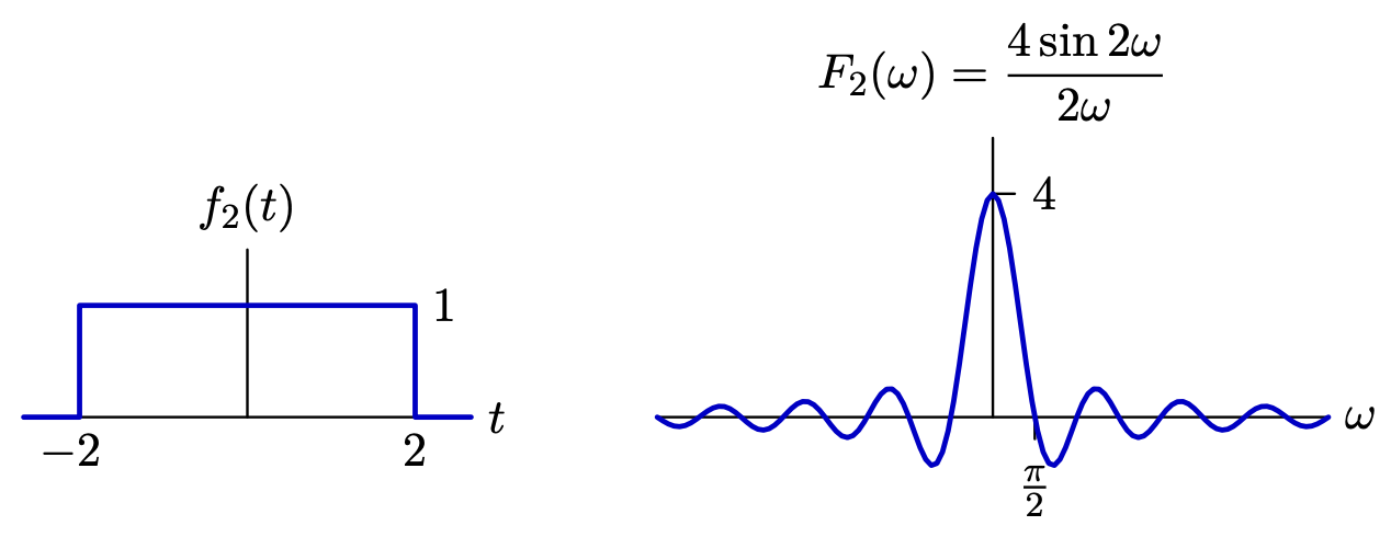
Our goal is to write Fourier series for aperiodic signals. Here's our prototypical example.

f(t) := \begin{cases} 1 & \text{ if } t \in (-1, 1). \\ 0 & \text{ otherwise.} \end{cases}

The guiding intuition is that all signals are technically periodic—it's just that the period of an aperiodic signal is $T \to \infty$ . Instead of a discrete sum $\sum_{k = -\infty}^{\infty} F[k] e^{jkt \omega_0}$ , we'll write $f$ as a continuous integral $\int_{-\infty}^{\infty} F(\omega) e^{jt \omega} \, \mathrm{d}\omega$ .

But let's take things slow. To build up to being able to say that $f(t)$ has period $T \to \infty$ , let's start by considering what happens when we force $f(t)$ to have some finite period $T$ by constructing an alternative $f_T(t)$ .

f_T(t) := \begin{cases} 1 & \text{ if } (t \% T) \in (-1, 1). \\ 0 & \text{ otherwise.} \end{cases}

As a function of $T$ , we now determine the array of Fourier coefficients $F_T$ for the periodic signal $f_T(t)$ .

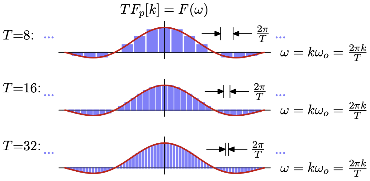
F_T[k] = \frac{1}{T} \int_{-1}^1 e^{-jt(\textcolor{#bf0140}{2\pi k/T})} \, \mathrm{d}t = \frac{1}{T} \left[ \frac{e^{-jt(\textcolor{#bf0140}{2\pi k/T})}}{-j(\textcolor{#bf0140}{2\pi k/T})} \right]_{-1}^{1} = \frac{1}{T} \cdot \frac{2\sin\left(\textcolor{#bf0140}{2\pi k/T}\right)}{(\textcolor{#bf0140}{2\pi k/T})}.

And here's a plot of $T \cdot F_T[k] = \frac{2\sin\left(\textcolor{#bf0140}{2\pi k/T}\right)}{(\textcolor{#bf0140}{2\pi k/T})}$ for $T = 16$ and $T = 8$ . (Note that $k$ can be any integer, not just those pictured below.)

Remark. Convince yourself that doubling $T$ has the effect of halving the “height” and doubling the “width” of the raw coefficients $F_T[k]$ . If we wanted to “normalize” the graphs for $T = 16$ and $T = 8$ so they looked similar, we might instead graph, say, $T \cdot F_T[k]$ against $2\pi k/T$ …

And so our Fourier series for $f_T(t)$ looks like the following:

f_T(t) = \frac{1}{T} \sum_{k = -\infty}^{\infty} \frac{2\sin(\textcolor{#bf0140}{2\pi k/T})}{\textcolor{#bf0140}{2\pi k/T}} e^{jt(\textcolor{#bf0140}{2\pi k/T})}.

There's a reparametrization begging to be made here: $\textcolor{#bf0140}{\omega_k := 2\pi k/T}$ for each $k \in \mathbb{Z}$ . Note that $\Delta \omega := \omega_{k + 1} - \omega_k = 2\pi/T$ . Now we can send $T \to \infty$ and see what happens to the Fourier series.

\begin{align*}f(t) = \lim_{T \to \infty} f_T(t) & = \lim_{T \to \infty} \frac{1}{T} \sum_{k = -\infty}^{\infty} \frac{2\sin(\textcolor{#bf0140}{2\pi k/T})}{\textcolor{#bf0140}{2\pi k/T}} e^{jt(\textcolor{#bf0140}{2\pi k/T})} \\ & = \lim_{T \to \infty} \frac{1}{2\pi} \sum_{k = -\infty}^{\infty} \frac{2\sin(\textcolor{#bf0140}{\omega_k})}{\textcolor{#bf0140}{\omega_k}} e^{jt \textcolor{#bf0140}{\omega_k}} \Delta \omega = \frac{1}{2\pi}\int_{-\infty}^{\infty} \frac{2\sin(\omega)}{\omega} e^{jt \omega} \, \mathrm{d}\omega.\end{align*}

And so our Fourier series now becomes a Fourier integral!

§ Lecture: The CT Fourier Transform

Naturally, we'd like to generalize: what's the relationship between $f(t)$ and $F(\omega) = \frac{2\sin(\omega)}{\omega}$ , and vice versa?

Theorem. (Fourier Transform) Given a CT signal $f(t)$ , define its Fourier transform to be $F(\omega) := \int_{-\infty}^{\infty} f(t) e^{-j\omega t} \, \mathrm{d}t$ . It then follows that $f(t) = \frac{1}{2\pi} \int_{-\infty}^{\infty} F(\omega) e^{jt \omega} \, \mathrm{d}\omega$ .

Proof: Follow the same recipe as before. Let $f_T(t)$ denote the extension of $f(t)$ to have period $T$ . Then its Fourier series is:

F_T[k] = \frac{1}{T} \int_T f(t) e^{-jt(\textcolor{#bf0140}{2\pi k/T})} \, \mathrm{d}t

In our prototypical example, we picked $F(\omega) = \frac{2\sin(\omega)}{\omega}$ so that $F(\omega) := \lim_{T \to \infty} T \cdot F_T[k]$ , where $\textcolor{#bf0140}{\omega = 2\pi k/T}$ . Let's follow the recipe and see what happens.

F(\omega) = \lim_{T \to \infty} T \cdot \left(\frac{1}{T} \int_T f(t) e^{-jt(\textcolor{#bf0140}{2\pi k/T})} \, \mathrm{d}t\right) = \lim_{T \to \infty} \int_T f(t) e^{-jt\textcolor{#bf0140}{\omega}} \, \mathrm{d}t = \int_{-\infty}^{\infty} f(t) e^{-jt\textcolor{#bf0140}{\omega}} \, \mathrm{d}t.

Just as promised. With $F(\omega)$ defined this way, watch what happens when we take the Fourier series of $f(t)$ and send $T \to \infty$ .

\begin{align*}f(t) = \lim_{T \to \infty} f_T(t) & = \lim_{T \to \infty} \sum_{k = -\infty}^{\infty} F_T[k] e^{jt(\textcolor{#bf0140}{2\pi k/T})} \\ & = \frac{1}{2\pi} \lim_{T \to \infty} \sum_{k = -\infty}^{\infty} F(\omega_k) e^{jt(\textcolor{#bf0140}{\omega_k})} \Delta \omega = \frac{1}{2\pi}\int_{-\infty}^{\infty} F(\omega) e^{jt\omega} \, \mathrm{d}\omega.\end{align*}

Just as promised. $\blacksquare$

Remark. Comparing and contrasting periodic and aperiodic signals…

All the frequencies in a periodic signal are captured in one period $\left(\int_T\right)$ , whereas aperiodic signals need all of $\mathbb{R}$ $\left(\int_{-\infty}^{\infty}\right)$ .
Periodic signals have a discrete set of frequencies $\left(\sum_{k = -\infty}^{\infty}\right)$ , whereas aperiodic signals have a continuous set $\left(\int_{-\infty}^{\infty} \, \mathrm{d}\omega\right)$ .

Importantly, there is now a clearer dual relationship between $f(t)$ and $F(\omega)$ . If the equation $F(\omega) := \int_{-\infty}^{\infty} f(t) e^{-j\omega t} \, \mathrm{d}t$ represents a Fourier transform, then the equation $f(t) = \frac{1}{2\pi} \int_{-\infty}^{\infty} F(\omega) e^{jt \omega} \, \mathrm{d}\omega$ represents an inverse Fourier transform.

Theorem. (Time-Frequency Duality) If the Fourier transform of $f(t)$ is $F(\omega)$ , then the Fourier transform of $F(t)$ is $2\pi f(-\omega)$ .

Proof: Just look at the formulas. $\blacksquare$

§ Lecture and Recitation: Properties of the CT Fourier Transform

Theorem. (Time Delay) The FT of $f(t - \tau)$ is $e^{-j \omega \tau} F(\omega)$ , and the inverse FT of $F(\omega - \omega_0)$ is $e^{jt \omega_0}f(t)$ .

Proof: True by inspecting the relationship $F(\omega) := \int_{-\infty}^{\infty} f(t) e^{-j\omega t} \, \mathrm{d}t$ . $\blacksquare$

Note that this suggests that our prototypical example was special in having a real-valued Fourier transform. Here's why.

Theorem. (Even / Odd) If $f(t)$ is real and even, $F(\omega)$ is real and even. If $f(t)$ is real and odd, $F(\omega)$ is imaginary and odd.

Proof: Again, true by inspecting the relationship $F(\omega) := \int_{-\infty}^{\infty} f(t) e^{-j\omega t} \, \mathrm{d}t$ . Another reason to see why is to apply the same argument as used for periodic signals; even signals are sums of pure cosines, and odd signals are sums of pure sines. $\blacksquare$

More generally, we can say the following:

Theorem. (Hermitian Symmetry) If $f(t)$ is real, then $F(-\omega) = \overline{F(\omega)}$ for all $\omega$ .

Proof: Again, just inspect the relationship $F(\omega) := \int_{-\infty}^{\infty} f(t) e^{-j\omega t} \, \mathrm{d}t$ . $\blacksquare$

We can also say that stretching a CT signal in one direction will cause its Fourier transform to stretch in the other direction.

Theorem. (Time Scaling) The FT of $f(at)$ is $\frac{1}{|a|}F\left(\frac{\omega}{a}\right)$ , and the inverse FT of $F(a\omega)$ is $\frac{1}{|a|}f\left(\frac{1}{a}t\right)$ .

Proof: Again, just inspect the relationship $F(\omega) := \int_{-\infty}^{\infty} f(t) e^{-j\omega t} \, \mathrm{d}t$ . The absolute value signs $|a|$ are necessary because when $a$ is negative, the $u$ -substitution $u = at$ causes the bounds of the integral to flip.

Alternatively, we can argue heuristically. This relationship says that, say, doubling the width of $f(t)$ causes its FT to shrink in width and double in height.

This should make sense; the signal $f(t/2)$ can be thought of as “playing back the signal $f(t)$ at $\times 0.5$ speed”, so the frequencies prominent in $f(t/2)$ should be half of those prominent in $f(t)$ . (And to balance it out, all frequency strengths are doubled.) $\blacksquare$

Here's some intuition as to why “balancing it out” is necessary.

Theorem. (FT Areas) The area under the curve of $f(t)$ is $F(0)$ , and the area under the curve of $F(\omega)$ is $2\pi f(0)$ .

Proof: Immediate from plugging in $t = 0$ or $\omega = 0$ as needed. $\blacksquare$

Finally, here's a property whose frequency half doesn't have an analogue for Fourier series.

Theorem. (Derivative FTs) The FT of $\frac{d}{dt} f(t)$ is $j\omega F(\omega)$ , and the inverse FT of $\frac{d}{d\omega} F(\omega)$ is $-jt f(t)$ .

Proof: This one is trickier. To show the FT of $\frac{d}{dt} f(t)$ is $j\omega F(\omega)$ , differentiate the synthesis equation.

\frac{d}{dt} f(t) = \frac{d}{dt} \frac{1}{2\pi} \int_{-\infty}^{\infty} F(\omega) e^{jt\omega} \, \mathrm{d}\omega = \frac{1}{2\pi} \int_{-\infty}^{\infty} j\omega F(\omega) e^{jt\omega} \, \mathrm{d}\omega.

To show inverse FT of $\frac{d}{d\omega} F(\omega)$ is $-jt f(t)$ , differentiate the analysis equation.

\frac{d}{d\omega} F(\omega) = \frac{d}{d\omega} \int_{-\infty}^{\infty} f(t) e^{-jt \omega} \, \mathrm{d}t = \int_{-\infty}^{\infty} -jt f(t) e^{-jt \omega} \, \mathrm{d}t. ~~~ \blacksquare

§ Lecture: The Dirac Delta Function

Consider our prototypical function $f(t)$ from earlier. Imagine compressing $f(t)$ inward by a factor of $A$ , producing functions like:

f_A(t) := \begin{cases} A & \text{ if } t \in \left(-\frac{1}{A}, \frac{1}{A}\right) \\ 0 & \text{ otherwise.} \end{cases}

Then the area under the curve of $f_A(t)$ is constantly $2$ , so $F_A(0)$ must be constantly $2$ . According to “Time Scaling”, in fact, the effect is that $F_A(\omega)$ “stretches outward” as $A$ tends to infinity, while still maintaining a $y$ -intercept of $2$ .

At the limit of $A \to \infty$ , we discover the following (up to a factor of $2$ ).

Theorem. (Dirac Delta FT) Let the Dirac delta function $\delta(t)$ be defined so that $\delta(t) = 0$ for all $t \neq 0$ and $\int_{-\infty}^{\infty} \delta(t) \, \mathrm{d}t = 1$ . Then the FT of $\delta(t)$ is the constant function $F(\omega) = 1$ .

The dual also holds: the FT of the constant function $f(t) = 1$ is $F(\omega) = 2\pi \delta(\omega)$ .

Proof: This follows from the heuristic argument from earlier. You can also formally verify this using the FT equations. $\blacksquare$

The Dirac delta function also appears when taking the Fourier transform of a periodic signal.

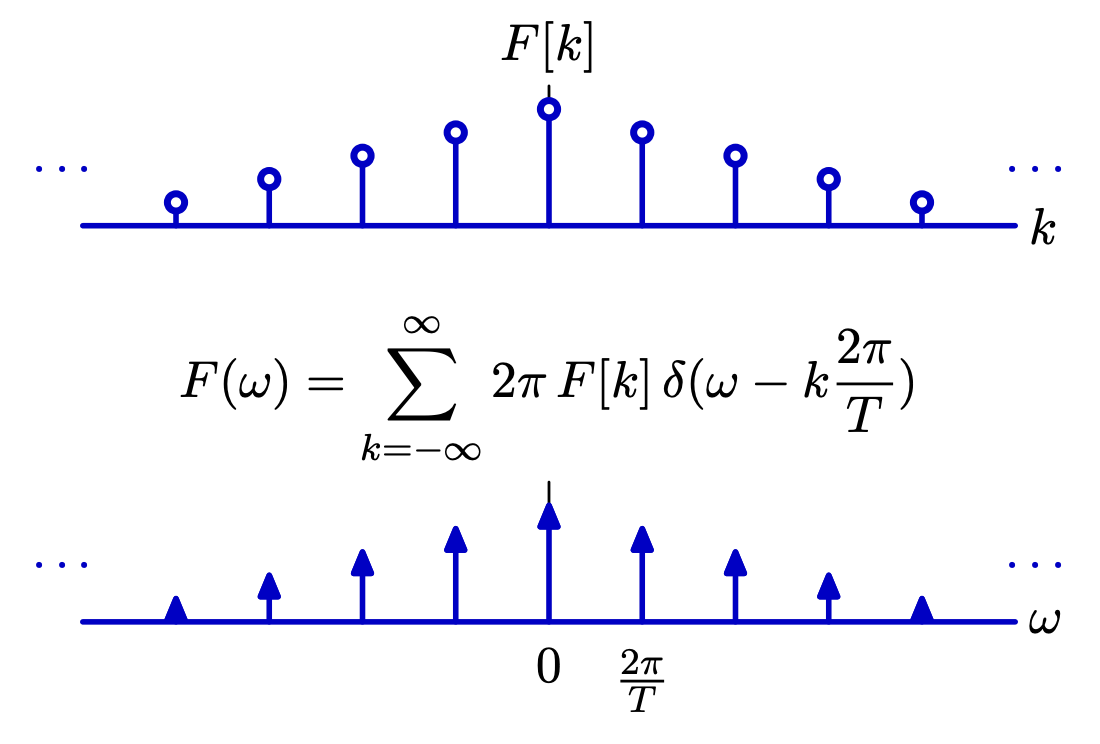
Theorem. (Periodic FT) Suppose $f(t)$ is a periodic signal with Fourier coefficients $F[k]$ , so that $f(t) = \sum_{k = -\infty}^{\infty} F[k] e^{jt(2\pi k/T)}$ . Then the Fourier transform of $f(t)$ is $F(\omega) = \sum_{k = -\infty}^{\infty} 2\pi F[k] \delta\left(\omega - \frac{2\pi k}{T}\right)$ .

Proof: Nicely, the FT is linear, so it suffices to find the FT of $F[k] e^{jt(2\pi k/T)}$ . This can be done nicely via “Time Delay”.

This should also just heuristically make sense: integrating over a discrete set of Dirac deltas is the same as summing over a discrete set of complex exponentials. $\blacksquare$