MIT 6.300 — Lecture 11

Communication Systems

The content of this lecture is not needed for future lectures, but it's a nice payoff of everything built up over the past ten lectures, explaining clever applications of signal processing techniques in the context of radio transmission.

§ Lecture: Wireless Communication (is Hard)

One way to interpret the signals we've been studying so far is to view them as functions of air pressure at a certain location over time. In this sense, one might physically produce a signal by, say, clapping your hands or shouting.

Another way to interpret a signal, however, is as a function of the strength of the electromagnetic field at a certain location over time. In this sense, one might physically produce a signal by using an antenna:

Fact. (Physics) In an antenna, electrons oscillate back and forth along its length; to achieve resonance, the wavelength of the signal produced by an antenna must be on the order of the antenna's length.

To communicate with someone, you might use your voice to produce an air pressure signal. But this form of communication has some disadvantages: it doesn't work over long distances, and it's not very private.

What if we tried communicating by using an antenna to send an electromagnetic signal instead?

Problem. We have a signal that represents human speech, containing frequencies from 200 Hz to 3000 Hz. We would like to communicate this signal wirelessly by transmitting and receiving electromagnetic waves via antenna.

How long must such an antenna be to transmit a 200–3000 Hz signal?

Solution: According to physics, a 200 Hz signal would have the longest wavelength, that being:

\lambda = \frac{c}{f} = \frac{3 \times 10^8 \ \text{m/s}}{200 \ \text{Hz}} = 1.5 \times 10^6 \ \text{m} = 1500 \ \text{km}.

Also according to physics, the optimal length of an antenna is on the order of the wavelength of the signal it seeks to transmit. So we would need an antenna $1500$ kilometers long…

The issue, of course, is that most antennas are $10$ centimeters long, not $1500$ kilometers.

Problem. What frequencies would be produced by an antenna that is $10$ centimeters long?

Solution: Again by physics, we would expect frequencies on the order of $f = \frac{c}{\lambda} \sim \frac{3 \times 10^8 \ \text{m/s}}{10 \ \text{cm}} \approx 3 \ \text{GHz}$ .

The challenge is that most signals (not just speech!) have frequencies that are not at all close to $3$ GHz.

If we want to communicate meaningful electromagnetic signals via antenna, we need to find some way to modulate these signals so that their frequencies fit within the desired range.

§ Lecture: Amplitude Modulation

To increase the frequencies present within a CT signal, we might hope to just, say, shift its Fourier transform to the right, like so:

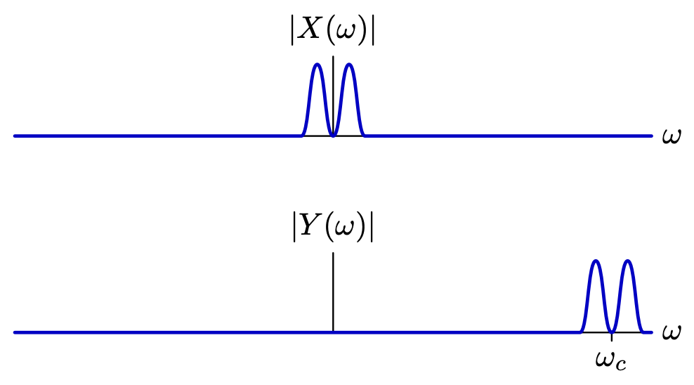
Recall from Lecture 6 that the effect of this is that $y(t) = e^{j \omega_c t} x(t)$ . By picking a large enough $\omega_c$ , we can bring the frequencies of $y(t)$ close to $3$ GHz, fixing our antenna-feasibility problem.

But this naive solution won't work as stated—the resulting signal $y(t)$ is complex-valued, and thus not physically transmittable! One easy way to see why is to note that $Y(\omega)$ doesn't satisfy Hermitian symmetry: $Y(-\omega) \neq \overline{Y(\omega)}$ .

The fix is to enforce Hermitian symmetry by redefining $Y(\omega)$ like so:

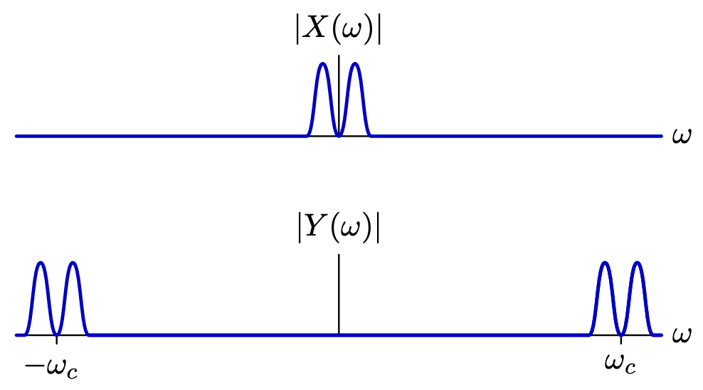
The effect of the above is that $y(t) = 2\cos(\omega_c t) x(t)$ , which is real-valued. In the time domain, you can see how $y(t)$ has a very high frequency for large $\omega_c$ , yet still communicates the “shape” of $x(t)$ .

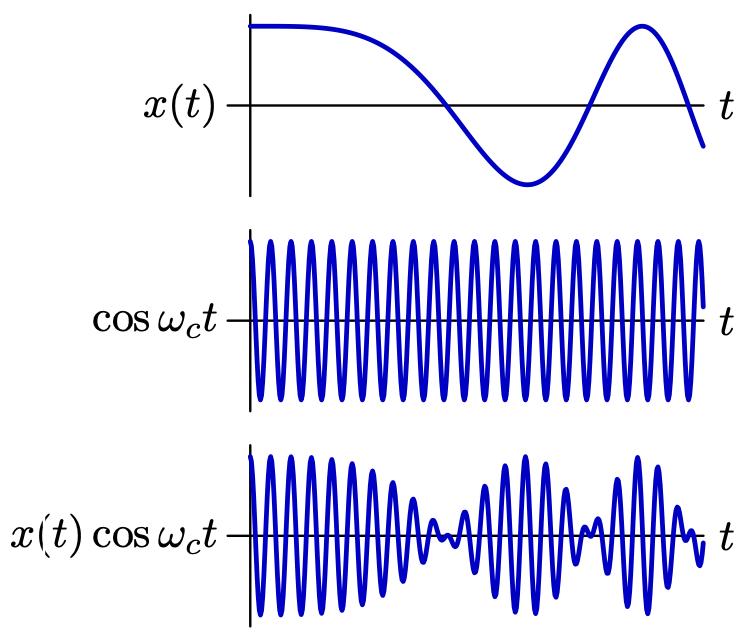
Definition. The system $x(t) \mapsto \cos(\omega_c t) x(t)$ is called amplitude modulation. (Note that we drop the factor of $2$ here.)

Remark. Note that amplitude modulation is not an LTI system: it's not time-invariant!

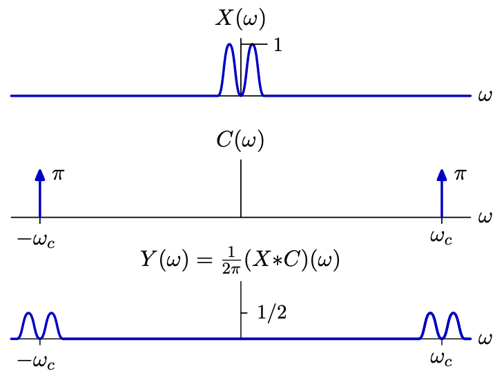
Additionally, note that we switched from $y(t) = 2\cos(\omega_c t) x(t)$ to $y(t) = \cos(\omega_c t) x(t)$ , dropping the factor of $2$ . The effect of this is that the amplitudes in $Y(\omega)$ will be half of those in $X(\omega)$ . We'll account for this later.

Here's another way to see why amplitude modulation affects the frequency domain in the way it does.

Theorem. (Filtering Dual) If $z(t) = x(t) \cdot y(t)$ , then $Z(\omega) = \frac{1}{2\pi} (X * Y)(\omega)$ . The same goes for DT signals.

Proof: This is the dual of the statement that the Fourier transform of a convolution equals the product of the Fourier transforms.

Here's the full computations written out for reference; there's nothing new here.

\begin{align*}Z(\omega) & = \int_{t = -\infty}^{\infty} x(t) y(t) e^{-j \omega t} \, \mathrm{d}t \\ & = \int_{t = -\infty}^{\infty} x(t) \left[ \frac{1}{2\pi} \int_{\lambda = -\infty}^{\infty} Y(\lambda) e^{j \lambda t} \, \mathrm{d}\lambda \right] e^{-j \omega t} \, \mathrm{d}t \\ & = \frac{1}{2\pi} \int_{\lambda = -\infty}^{\infty} Y(\lambda) \left[ \int_{t = -\infty}^{\infty} x(t) e^{-j(\omega - \lambda)t} \, \mathrm{d}t \right] \, \mathrm{d}\lambda \\ & = \frac{1}{2\pi} \int_{\lambda = -\infty}^{\infty} Y(\lambda) \left[ X(\omega - \lambda) \right] \, \mathrm{d}\lambda = \frac{1}{2\pi}(X * Y)(\omega).\end{align*}

And the same goes for DT signals, as expected. $\blacksquare$

And so the point is that multiplying $x(t)$ by $c(t) := \cos(\omega_c t)$ is the same as convolving $X(\omega)$ with the Fourier transform $C(\omega) := \pi \cdot \left( \delta(\omega - \omega_c) + \delta(\omega + \omega_c) \right)$ and dividing the result by $2\pi$ , which has the effect shown below.

§ Lecture: Synchronous Demodulation

After transmitting the modulated signal $y(t) = x(t) \cos(\omega_c t)$ , what happens on the receiving end—how can we demodulate $y(t)$ to retrieve the original signal $x(t)$ ? The answer is…

Definition. The system $y(t) \mapsto \cos(\omega_c t) y(t)$ is called synchronous demodulation.

Yes, that is the exact same system as amplitude modulation. Nonetheless, it works!

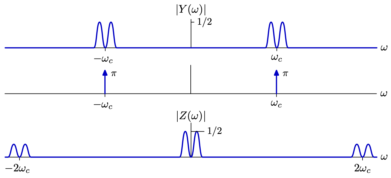
After receiving $y(t)$ , we simply apply synchronous demodulation, then apply a low-pass filter, and finally multiply the result by $2$ . The diagram above explains why this works in the frequency domain, but you can justify it in the time domain, too:

z(t) = \cos(\omega_c t) y(t) = \cos^2(\omega_c t) x(t) = \left(\frac{1}{2} + \frac{1}{2}\cos(2\omega_c t)\right) x(t).

Applying a low-pass filter to $z(t)$ deletes the $\frac{1}{2}\cos(2\omega_c t) x(t)$ term, leaving behind just the original signal $\frac{1}{2}x(t)$ .

§ Lecture: Multiple Transmitters

This protocol comes built-in with a neat feature: it allows a single receiver to listen to multiple transmitters at once, as long as each transmitter uses a different choice of $\omega_c$ .

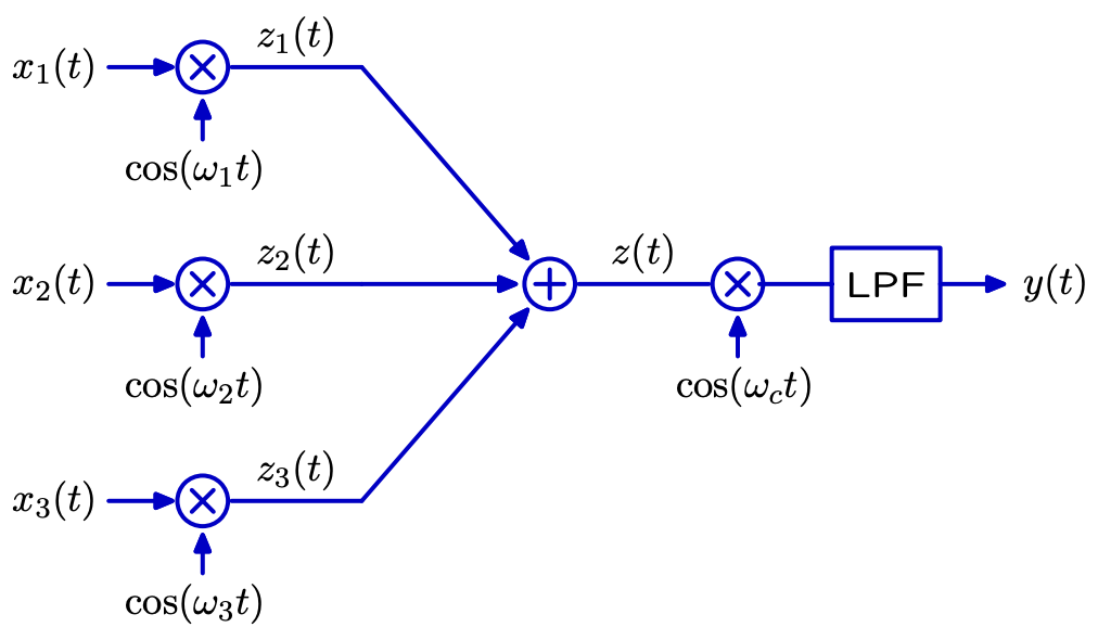
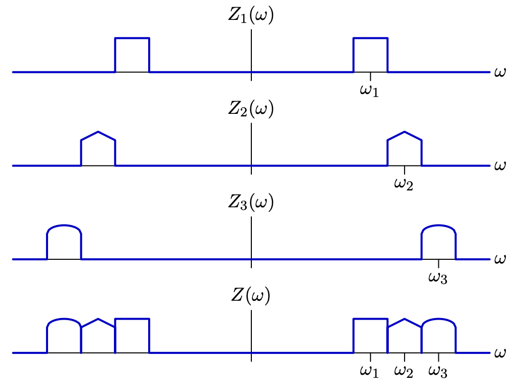
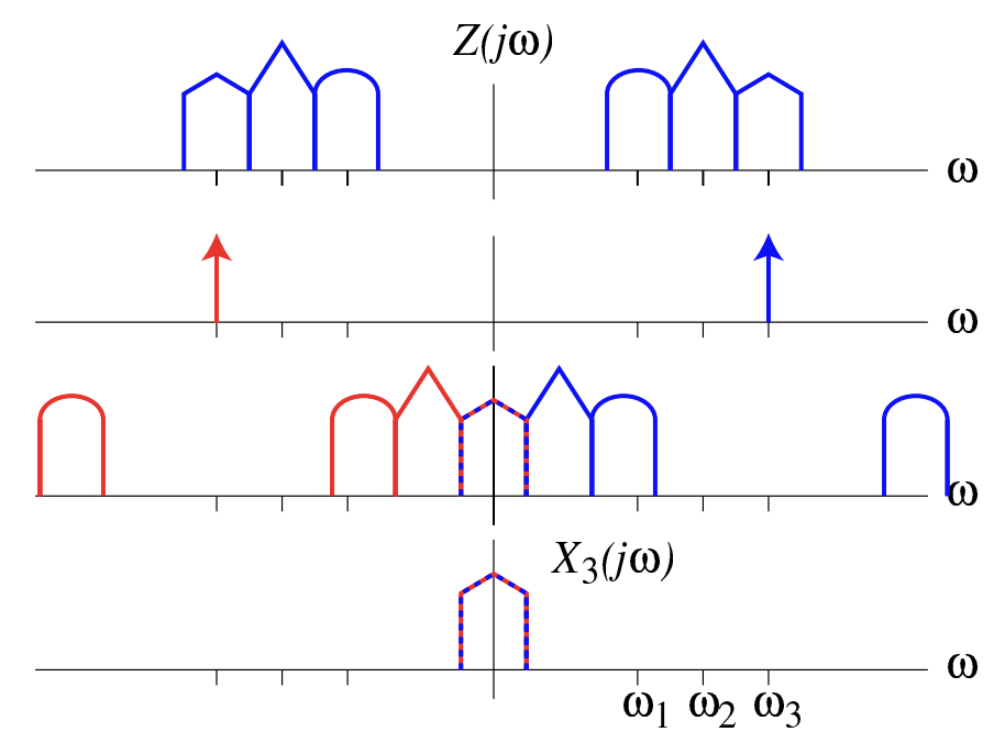
In the above, by specifying the frequency $\omega_c$ to use for synchronous demodulation, the output signal $y(t)$ can be set to read from any of $x_1(t)$ , $x_2(t)$ , or $x_3(t)$ . Setting $\omega_c = \omega_2$ , for example, would yield $y(t) = \frac{1}{2} x_2(t)$ .

To demonstrate this, here's what the summed-together signal $z(t)$ looks like in the frequency domain.

And here's how setting $\omega_c = \omega_3$ allows the output signal $y(t)$ to match $x_3(t)$ , as shown in the frequency domain.

Remark. Ever hear of AM radio before? It refers to the first type of audio broadcasting technology ever made. And the AM stands for amplitude modulation.

§ Lecture: Amplitude Modulation with Carrier

Importantly, the carrier signal $\cos(\omega_c t)$ used in amplitude modulation must match the carrier signal $\cos(\omega_c t)$ used in synchronous demodulation. What happens if the two carrier signals used differ by a phase shift $\phi$ , though?

\begin{align*}z(t) & = \cos(\omega_c t) \cos(\omega_c t + \phi) \cdot x(t) \\ & = \frac{1}{2} \left[\cos(\phi) + \cos(2 \omega_c t + \phi)\right] \cdot x(t) \\ & = \frac{1}{2} x(t) \cos(\phi) + \frac{1}{2}x(t) \cos(2 \omega_c t + \phi).\end{align*}

The latter of the two RHS terms will get filtered out via the LPF. But the former of those two terms $\frac{1}{2}x(t) \cos(\phi)$ might experience fading for unlucky values of $\phi$ (say, $\phi \approx \frac{\pi}{2}$ ).

Let's consider an entirely new approach to modulation and demodulation that bypasses this issue.

Approach (AM with Carrier). Suppose we wish to transmit a signal $x(t)$ using an antenna.

Pick a very high frequency $\omega_c$ , along with a constant $C > |x(t)|$ .
Use the antenna to transmit the E/M wave $z(t) := \left(x(t) + C\right) \cos(\omega_c t)$ .
On the receiving end, apply a peak detector to $z(t)$ and subtract $C$ to retrieve the original signal $x(t)$ .

Notice how this approach doesn't even use synchronous demodulation; the demodulation is the peak detector itself.

To understand why this new protocol works, consider the shape of the transmitted signal $z(t)$ .

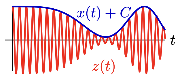
The signal $z(t)$ that is transmitted has a special property: its shape (formally, “envelope”) traces out the shape of $x(t) + C$ . Note that this property relies on the assumption that $C > |x(t)|$ .

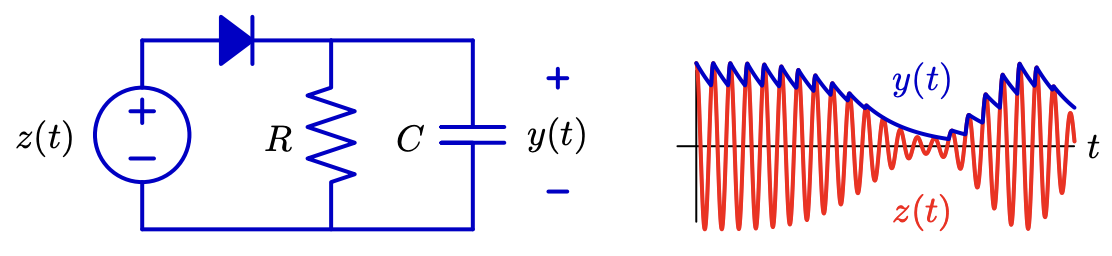
On the receiving end, reading out that “envelope” is not very hard to do in hardware: all it takes is a single RC circuit (our peak detector). Thus, the receiver just has to read the envelope $y(t)$ , then subtract $C$ to retrieve $x(t) \approx y(t) - C$ .

One downside of this approach is that it doesn't make use of synchronous demodulation; the receiver can't distinguish between multiple transmissions added together, even if each transmitter uses a different value for $\omega_c$ . (A band-pass filter that first isolates a single transmission would fix this—that's what real AM radios do.)

Another downside of this approach is the power necessary to produce the E/M wave $z(t) := x(t) \cos(\omega_c t) + C \cos(\omega_c t)$ .

Problem. Compare the power of the E/M wave $z(t) = x(t) \cos(\omega_c t) + C \cos(\omega_c t)$ to that of $x(t) \cos(\omega_c t)$ .

Solution: Let's say $x_{\mathrm{p}}$ is the peak value of $x(t)$ , and $x_{\mathrm{rms}}$ is the root-mean-square value of $x(t)$ .

According to physics, the power carried by $x(t) \cos(\omega_c t)$ is proportional to $x_{\mathrm{rms}}^2$ .
Note that we require $C > x_{\mathrm{p}}$ . According to physics, the power carried by $C \cos(\omega_c t)$ is proportional to $C^2 > x_{\mathrm{p}}^2$ .

The unfortunate fact, however, is that typically $x_{\mathrm{p}} > 35 \cdot x_{\mathrm{rms}}$ .

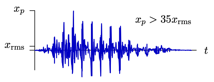
So the power needed to transmit the carrier tends to be more than $1225$ times the power needed to transmit the message itself. This is an acceptable tradeoff for 50 kW broadcast radio, perhaps, but not for, say, phone calls and cell phone batteries.

There are, of course, technologies developed to fix some of these issues; we won't get into those details.

§ Recitation: Implementing Band-Pass Filters (BPFs)

Recalling Lecture 10, we already have designed systems that function as low-pass filters. Now let's design a band-pass filter instead: a filter that accepts frequencies within some margin $\pm \Omega_d$ of either $\Omega_c$ or $-\Omega_c$ .

Remark. As a reminder, we are working with DT signals, so all frequencies $\Omega$ are to be interpreted modulo $2\pi$ .

Here's one strategy that's sure to work.

Theorem. (BPF #1) Let $h_{\mathrm{LPF}}[n]$ denote the unit-sample response of a low-pass filter with cutoff frequency $\Omega_d$ . Then a system whose unit-sample response is $h[n] := h_{\mathrm{LPF}}[n] \cdot \cos(\Omega_c n)$ is a band-pass filter.

Proof: We would like the frequency response $H(\Omega)$ of our BPF system to look like two copies of that of an LPF system, one centered at $\Omega = -\Omega_c$ , and another centered at $\Omega = \Omega_c$ .

To construct such a frequency response, let's just steal an idea from amplitude modulation.

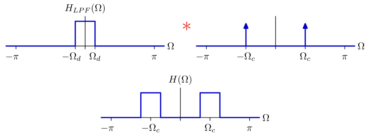
It suffices to take the frequency response $H_{\mathrm{LPF}}(\Omega)$ of the LPF, convolve it with $C(\Omega) := \pi \cdot \left( \delta(\Omega - \Omega_c) + \delta(\Omega + \Omega_c) \right)$ , and divide by $2\pi$ . But just as with amplitude modulation (see the “Filtering Dual” theorem from earlier), convolving with $C(\Omega)$ and dividing by $2\pi$ is the same as multiplying by $c[n] := \cos(\Omega_c n)$ .

So we want $h[n] = h_{\mathrm{LPF}}[n] \cdot c[n] = h_{\mathrm{LPF}}[n] \cdot \cos(\Omega_c n)$ . $\blacksquare$

Instead of defining such a system by its unit-sample response, however, let's try defining it in the time domain.

Theorem. (BPF #2) The BPF we seek is described by the cascading system depicted below.

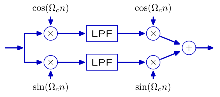
Proof: Recalling the relationship between a system and its unit-sample response from Lecture 9, we can directly read off:

\begin{align*}y[n] & = (x * h)[n] \\ & = \sum_{m = -\infty}^{\infty} x[m] \cdot h_{\mathrm{LPF}}[n - m] \cos(\Omega_c(n - m)) \\ & = \sum_{m = -\infty}^{\infty} x[m] \cdot h_{\mathrm{LPF}}[n - m] \left(\cos(\Omega_c n) \cos(\Omega_c m) + \sin(\Omega_c n) \sin(\Omega_c m)\right) \\ & = \underbrace{\left( \sum_{m = -\infty}^{\infty} x[m] \cos(\Omega_c m) \cdot h_{\mathrm{LPF}}[n - m] \right)}_{ x[n] \cos(\Omega_c n) \ * \ h_{\mathrm{LPF}}[n] } \cdot \cos(\Omega_c n) + \underbrace{\left( \sum_{m = -\infty}^{\infty} x[m] \sin(\Omega_c m) \cdot h_{\mathrm{LPF}}[n - m] \right)}_{ x[n] \sin(\Omega_c n) \ * \ h_{\mathrm{LPF}}[n] } \cdot \sin(\Omega_c n)\end{align*}

And the above is exactly what the cascading system above computes. $\blacksquare$

Philosophically, here's one way to think about what the system above is actually accomplishing.

Philosophy of BPF #2. The input $X(\Omega)$ has two sections we wish to keep: the section $X_+$ over the band $[+\Omega_c \pm \Omega_d]$ , and the section $X_-$ over the band $[-\Omega_c \pm \Omega_d]$ . (Throughout this discussion, we'll ignore constant factors like $\frac{1}{2}$ .)

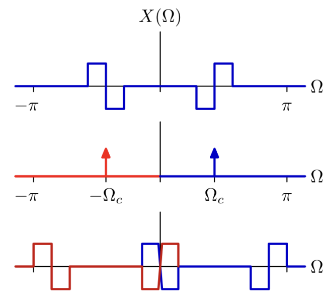
Here's what happens to $X(\Omega)$ when we multiply $x[n]$ by $\cos(\Omega_c n)$ and apply an LPF.

In doing so, we isolate the sum of $X_+$ and $X_-$ in the middle of the resulting spectrum.

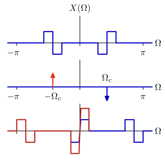
In contrast, here's what happens to $X(\Omega)$ when we multiply $x[n]$ by $\sin(\Omega_c n)$ and apply an LPF.

In this case, we isolate the difference of $X_+$ and $X_-$ instead. Here's the reason behind these two effects:

Multiplying $x[n]$ by $c[n] := \cos(\Omega_c n)$ is the same as…

… convolving $X(\Omega)$ with $C(\Omega) := \pi \cdot \left( \delta(\Omega - \Omega_c) + \delta(\Omega + \Omega_c) \right)$ and dividing by $2\pi$ .
Multiplying $x[n]$ by $s[n] := \sin(\Omega_c n)$ is the same as…

… convolving $X(\Omega)$ with $S(\Omega) := \frac{\pi}{j} \cdot \left( \delta(\Omega - \Omega_c) - \delta(\Omega + \Omega_c) \right)$ and dividing by $2\pi$ .

Neither the sum nor the difference of $X_+$ and $X_-$ are what we want, though. We want $X_+$ and $X_-$ each on their own, not their combination. But here's the point: the sum and the difference, together, are sufficient data for recovering each section individually! Here's how.

Multiplying the “sum-signal” by $\cos(\Omega_c n)$ deposits the sum $[X_+ + X_-]$ at both $+\Omega_c$ and $-\Omega_c$ .
Multiplying the “difference-signal” by $\sin(\Omega_c n)$ deposits $[X_+ - X_-]$ at $+\Omega_c$ and $[X_- - X_+]$ at $-\Omega_c$ .

Summing these deposits together then leaves $X_+$ back at $+\Omega_c$ and $X_-$ back at $-\Omega_c$ , exactly as desired.

§ Recitation: DSB-AM vs. SSB-SC

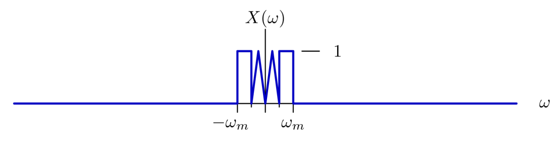
The $x(t) \cos(\omega_c t)$ transmission strategy—the first of the two we discussed—has a more complicated name: Double Sideband Amplitude Modulation (DSB-AM).

It's called Double Sideband because, in the frequency domain, the transform $X(\omega)$ appears twice in the output.
It's called amplitude modulation because, in the time domain, the signal $x(t)$ modulates the amplitude of $\cos(\omega_c t)$ .

The downside of DSB-AM is in the Double Sideband property—it seems to transmit twice as much data as it needs to.

There is an optimization to be made that can cut the cost of transmitting messages by a factor of two. Instead of using the wasteful amplitude modulation $x(t) \mapsto y(t) := \cos(\omega_c t) x(t)$ from earlier, we define $y(t)$ like so:

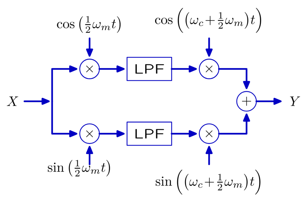
In the above, $\omega_m$ is a frequency such that the interval $[-\omega_m, \omega_m]$ captures all of the nonzero behavior of $X(\omega)$ .

Let's see why this new protocol—called SSB-SC, or Single-Sideband Suppressed-Carrier—actually works.

Remark. In what follows, we will (for the first time!) require the fact that $x(t)$ is real, meaning that $X(\omega)$ satisfies Hermitian symmetry. Note that this only guarantees $X(-\omega) = \overline{X(\omega)}$ , not that $X(\omega)$ is even! See Lecture 6.

Rather than transmitting a signal that deposits copies of $X(\omega)$ at $+\omega_c$ and $-\omega_c$ , our new protocol will deposit a copy of the right half of $X(\omega)$ at $+\omega_c$ , and the left half of $X(\omega)$ at $-\omega_c$ , like so.

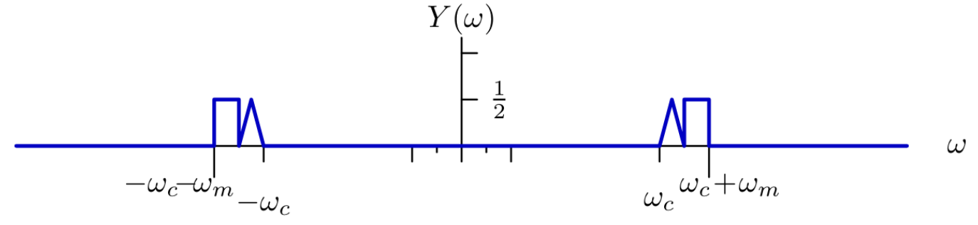
Remark. The name Single-Sideband Suppressed-Carrier makes sense: only a single sideband of $X(\omega)$ is kept on each side, and unlike “AM with Carrier,” no $C \cos(\omega_c t)$ carrier term is transmitted—the carrier is suppressed.

Note that we already need to be careful about validity here—we must check that $Y(\omega)$ is Hermitian symmetric, because if not, the corresponding signal $y(t)$ that we are trying to transmit will not be real-valued!

Fortunately, $Y(\omega)$ is Hermitian symmetric. But notice how this relies on $x(t)$ being real!

Now we study how the cascading system depicted above achieves the goal of SSB-SC promised here.

Philosophy of SSB-SC. Let $X_+$ denote the right half of $X(\omega)$ over the interval $[0, +\omega_m]$ , and let $X_-$ denote the left half of $X(\omega)$ over the interval $[-\omega_m, 0]$ . Just as in BPF #2, notice:

Multiplying $x(t)$ by $c(t) := \cos\left(\frac{1}{2}\omega_m t\right)$ and using an LPF is the same as…

… overlaying the sum $[X_+ + X_-]$ across the band $\left[-\frac{1}{2}\omega_m, \frac{1}{2}\omega_m\right]$ .
Multiplying $x(t)$ by $s(t) := \sin\left(\frac{1}{2}\omega_m t\right)$ and using an LPF is the same as…

… overlaying the difference $[X_+ - X_-]$ across the band $\left[-\frac{1}{2}\omega_m, \frac{1}{2}\omega_m\right]$ .

And just as before, the sum and the difference, together, are sufficient data for recovering each of $X_+$ and $X_-$ individually and depositing them at $+\omega_c$ and $-\omega_c$ , respectively.

Multiplying the “sum-signal” by $\cos\left((\omega_c + \frac{1}{2}\omega_m)t\right)$ deposits the sum $[X_+ + X_-]$ at both $+\omega_c$ and $-\omega_c$ .
Multiplying the “difference-signal” by $\sin\left((\omega_c + \frac{1}{2}\omega_m)t\right)$ deposits $[X_+ - X_-]$ at $+\omega_c$ and $[X_- - X_+]$ at $-\omega_c$ .

Summing these deposits together then leaves $X_+$ at $+\omega_c$ and $X_-$ at $-\omega_c$ , exactly as desired. (Here, “at $\pm\omega_c$ ” really means over the bands $[\omega_c, \omega_c + \omega_m]$ and $[-\omega_c - \omega_m, -\omega_c]$ , as in the goal diagram—the deposits are centered at $\pm(\omega_c + \frac{1}{2}\omega_m)$ .)